20 Tutorial 08 - Estimating Hydrodynamic Derivatives and Coefficients

Question 01

For a ship with \(L = 200\) m and \(U = 12\) m/s, analyze how the ratio of nonlinear to linear contributions in yaw moment changes as rudder angle increases from \(5^{\circ}\) to \(35^{\circ}\) in \(15^{\circ}\) increments. Use:

\(N'_\delta = 0.15\)
\(N'_{\delta\delta\delta} = 0.08\)

Question 02

A ship executes a turning maneuver where its yaw rate follows Nomoto’s model with \(T = 10\) s and \(K = 0.1\) /s. Assuming a constant rudder angle \(\delta = 10^\circ\):

Using initial heading \(\psi(0) = r(0) = 0\), calculate \(\psi(2)\) using:

Analytical integration
Euler scheme with \(h = 1\) s
RK4 scheme with \(h = 1\) s

Calculate the percentage error in heading angle at \(t = 1\) s for both numerical schemes

Question 03

Consider a ship of length \(L=180\) m, breadth \(B=30\) m, draft \(T=11\) m. If \(x_G = 0\) determine the block coefficient (upto 4 demcimals) at which the ship’s straight line stability characteristics change. You may assume the empirical formulas for the hydrdodynamic derivatives.

Question 04

A straight-line test at \(U=1.5\) m/s gives:

\(\beta\) (deg)	\(Y\) (N)
2	3.3
4	6.3
6	9.9
8	13.3
10	16.9

Compute \(Y_v\) using least squares fit through this data and compare it with the value obtained by computing slope numerically (using forward difference method) at the first data point.

Question 01 Solution

\(N'_\delta = 0.15\)
\(N'_{\delta\delta\delta} = 0.08\)

Code

import numpy as np

def solve_problem_1():
    N_delta = 0.15
    N_delta_delta_delta = 0.08
    L = 200
    U = 12

    delta_list = np.arange(5, 40, 15)
    delta_list_rad = np.deg2rad(delta_list)
    N_linear = N_delta * delta_list_rad
    N_nonlinear = N_delta_delta_delta * delta_list_rad**3
    ratio = N_nonlinear / N_linear
    print(f"The ratio of nonlinear to linear contributions in yaw moment changes from {ratio[0]*100:.2f} % at {delta_list[0]:.0f} deg to {ratio[1]*100:.2f} % at {delta_list[1]:.0f} deg and to {ratio[2]*100:.2f} % at {delta_list[2]:.0f} deg\n")

solve_problem_1()

The ratio of nonlinear to linear contributions in yaw moment changes from 0.41 % at 5 deg to 6.50 % at 20 deg and to 19.90 % at 35 deg

Question 02 Solution

A ship executes a turning maneuver where its yaw rate follows Nomoto’s model with \(T = 10\) s and \(K = 0.1\) /s. Assuming a constant rudder angle \(\delta = 10^\circ\):

Using initial heading \(\psi(0) = r(0) = 0\), calculate \(\psi(2)\) using:

Analytical integration
Euler scheme with \(h = 1\) s
RK4 scheme with \(h = 1\) s

Calculate the percentage error in heading angle at \(t = 1\) s for both numerical schemes

Code

import numpy as np

def solve_problem_2():
    T = 10
    K = 0.1
    delta = 10 * np.pi / 180
    h = 1
    t = 2

    # a)
    r_analytical = K * delta * (1 - np.exp(-t/T))
    psi_analytical = K * delta * (t - T * (1 - np.exp(-t/T)))
    print(f"The heading angle at t = {t} s using analytical solution is {psi_analytical*180/np.pi:.4f} degrees\n")
    
    # b)
    ss0 = np.array([0, 0])
    def f(t, ss):
        psi = ss[0]
        r = ss[1]        
        return np.array([r, (K * delta - r) / T])
    
    ss1 = ss0 + h * f(0, ss0)
    ss2 = ss1 + h * f(h, ss1)
    psi_euler = ss2[0]
    print(f"The heading angle at t = {t} s using Euler scheme is {psi_euler*180/np.pi:.4f} degrees\n")

    # c)
    k1 = f(0, ss0)
    k2 = f(h/2, ss0 + h/2 * k1)
    k3 = f(h/2, ss0 + h/2 * k2)
    k4 = f(h, ss0 + h * k3)
    ss1 = ss0 + h * (k1 + 2*k2 + 2*k3 + k4) / 6

    k1 = f(h, ss1)
    k2 = f(h + h/2, ss1 + h/2 * k1)
    k3 = f(h + h/2, ss1 + h/2 * k2)
    k4 = f(h + h, ss1 + h * k3)
    ss2 = ss1 + h * (k1 + 2*k2 + 2*k3 + k4) / 6
    psi_rk4 = ss2[0]
    print(f"The heading angle at t = {t} s using RK4 scheme is {psi_rk4*180/np.pi:.4f} degrees\n")
    
    # d)
    error_euler = np.abs(psi_euler - psi_analytical) / psi_analytical * 100
    error_rk4 = np.abs(psi_rk4 - psi_analytical) / psi_analytical * 100
    print(f"The percentage error in heading angle at t = {t} s using Euler scheme is {error_euler:.2f} %.\n")
    print(f"The percentage error in heading angle at t = {t} s using RK4 scheme is {error_rk4:.2f} %.\n")

solve_problem_2()

The heading angle at t = 2 s using analytical solution is 0.1873 degrees

The heading angle at t = 2 s using Euler scheme is 0.1000 degrees

The heading angle at t = 2 s using RK4 scheme is 0.1873 degrees

The percentage error in heading angle at t = 2 s using Euler scheme is 46.61 %.

The percentage error in heading angle at t = 2 s using RK4 scheme is 0.00 %.

Question 03 Solution

Code

import numpy as np

def solve_problem_3():
    L = 180
    B = 30
    T = 11
    
    xGp = 0

    
    Yrp = -np.pi * (T / L) ** 2 * (-0.5 + 2.2 * (B / L) - 0.08 * (B / T))
    Nvp = -np.pi * (T / L) ** 2 * (0.5 + 2.4 * (T / L))
    Nrp = -np.pi * (T / L) ** 2 * (1 / 4 + 0.039 * (B / T) - 0.56 * (B / L))

    C_B_limit = (np.pi * Nrp * (T/L)**2 + Nvp*Yrp) / (2*Nvp*B*T / L**2 - (0.4 * np.pi * (T/L)**2 * (B/T)) * Nrp)
    print(f"The ship is straight line stable for C_B < {C_B_limit:.4f}")

    # Yvp = -np.pi * (T / L) ** 2 * (1 + 0.4 * C_B_limit * (B / T))
    # mp = 2*C_B_limit * B * T / L**2
    # Cp = Yvp * (Nrp - mp * xGp) - Nvp * (Yrp - mp)
    # print(Cp)

solve_problem_3()

The ship is straight line stable for C_B < 0.5867

Question 04 Solution

A straight-line test at \(U=1.5\) m/s gives:

\(\beta\) (deg)	\(Y\) (N)
2	3.3
4	6.3
6	9.9
8	13.3
10	16.9

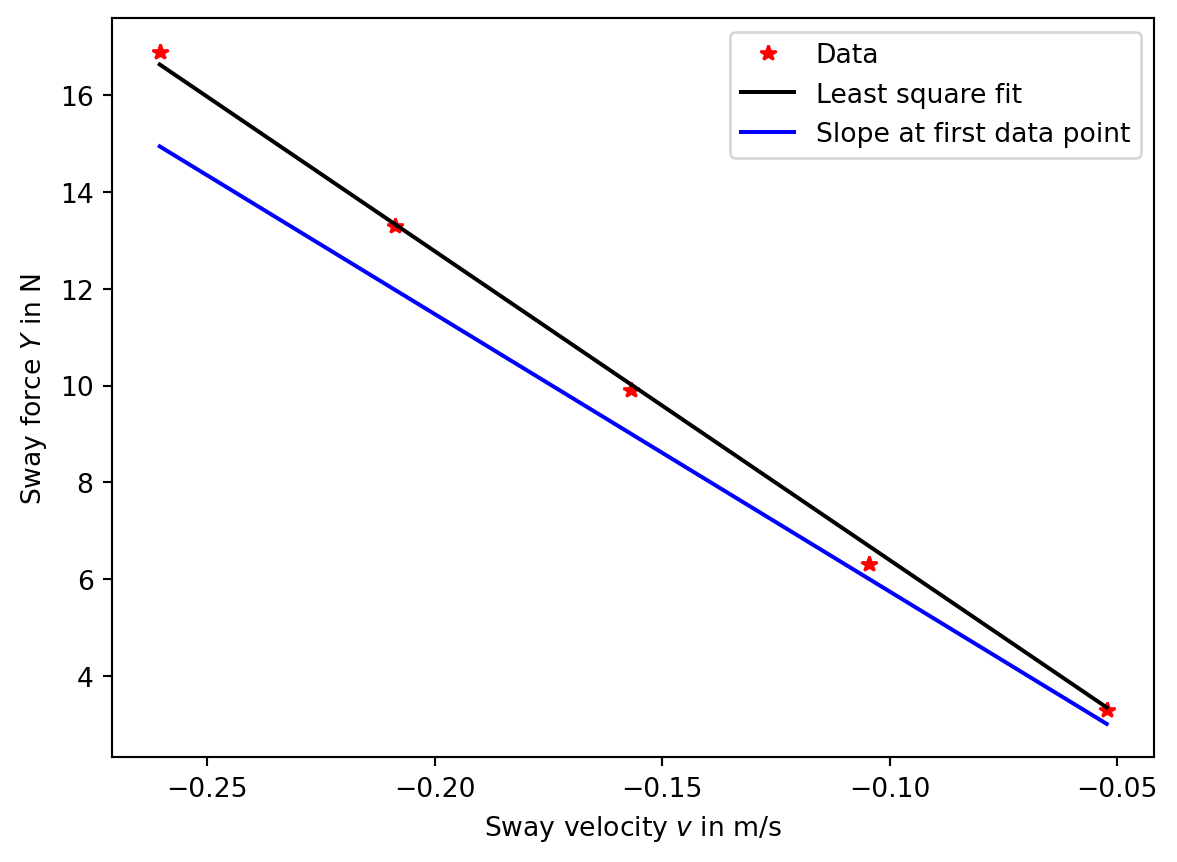
Compute \(Y_v\) using least squares fit through this data and compare it with the value obtained by computing slope numerically (using forward difference method) at the first data point.

Code

import numpy as np
import matplotlib.pyplot as plt

def solve_problem_4():

    U = 1.5
    bet = np.deg2rad(np.array([2, 4, 6, 8, 10]))
    Y = np.array([3.3, 6.3, 9.9, 13.3, 16.9])
    v = -np.sin(bet) * U

    Yv = np.sum(Y*v) / np.sum(v**2)
    print(f"Least square fit: {Yv:.2f}")

    slope0 = (Y[1] - Y[0])/(v[1] - v[0])

    print(f"Slope at first data point: {slope0:.2f}")
    
    plt.plot(v,Y,'r*',label='Data')
    plt.plot(v, Yv*v,'k', label='Least square fit')
    plt.plot(v, slope0*v,'b', label='Slope at first data point')
    
    plt.xlabel('Sway velocity $v$ in m/s')
    plt.ylabel('Sway force $Y$ in N')
    plt.legend()

solve_problem_4()

Least square fit: -63.88
Slope at first data point: -57.38