3 Linearized Maneuvering Equations
Note that the differential equations derived in the previous chapter are nonlinear in nature and are strongly coupled. This means that motion in one degree of freedom strongly affects the motion in other degrees of freedom. In general, it is difficult to find a closed form solution (analytical solutions) for such nonlinear equations. Although an alternative is to solve these equations numerically, numerical methods are computationally expensive and time consuming.
As most ships and underwater vehicles do not undertake sharp or fast maneuvers, we can assume that the difference between their instantaneous velocities and their values in a nominal operation are small. Leveraging on this assumption, the equations of motion can be linearized. Linear systems are a lot easier to understand than nonlinear systems. Specifically, the stability properties of a linear system are well understood and these properties can be determined without the need to numerically simulate the dynamics. Stability will be discussed in detail in the next chapter. Note that even when vehicles are designed for sharp maneuvers (like defense vehicles), the linearized system still provides a good starting point in designing the maneuvering characteristics of the vessel. This chapter will focus on the linearized maneuevering equations for a surface vessel and its stabilty characteristics.
In the nominal operating condition, a surface vessel or an underwater vehicle moves steadily forward with design speed \(U\). In this condition, the vessel does not experience any sway, heave, roll, pitch and yaw velocities. If the vessel does not undertake sharp maneuvers, it can be assumed that the sway, heave, roll, pitch and yaw velocities are small quantiities. It can also be assumed that the difference between the surge velocity and the design speed \(\Delta u = (u-U)\) is small. Thus the dynamic equations of motion in this case can be linearized about the nominal oprating condition and are shown in (\(\ref{eq-eom-expanded-1a}\) - \(\ref{eq-eom-expanded-6a}\)).
\[\begin{align} m\left[\dot{u} - y_G \dot{r} + z_G \dot{q}\right] = X \label{eq-eom-expanded-1a} \end{align}\]
\[\begin{align} m \left[\dot{v} - z_G \dot{p} + x_G \dot{r} + Ur \right] = Y \label{eq-eom-expanded-2a} \end{align}\]
\[\begin{align} m \left[\dot{w} - x_G \dot{q} + y_G \dot{p} - Uq \right] = Z \label{eq-eom-expanded-3a} \end{align}\]
\[\begin{align} I_x \dot{p} - \dot{r} I_{xz} - \dot{q} I_{xy} + m \left[y_G \dot{w} - y_G U q - z_G \dot{v} - z_G U r\right] = K \label{eq-eom-expanded-4a} \end{align}\]
\[\begin{align} I_y \dot{q} - \dot{p} I_{yx} - \dot{r} I_{yz} + m \left[z_G \dot{u} - x_G \dot{w} + x_G U q\right] = M \label{eq-eom-expanded-5a} \end{align}\]
\[\begin{align} I_z \dot{r} - \dot{q} I_{zy} - \dot{p} I_{zx} + m \left[x_G \dot{v} + x_G U r - y_G \dot{u} \right] = N \label{eq-eom-expanded-6a} \end{align}\]
In the matrix form the linearized dynamic equations can be expressed as shown in \(\eqref{eq-linearized-eom-matrix-compact}\), where \(\boldsymbol{L}_{RB}\) is the linearized Coriolis matrix and is shown in \(\eqref{eq-linearized-coriolis-matrix}\).
\[\begin{align} \boldsymbol{M}_{RB} \{\dot{v}\} + \boldsymbol{L}_{RB} \{v\} = \{\tau_{RB}\} \label{eq-linearized-eom-matrix-compact} \end{align}\]
\[\begin{align} \boldsymbol{L}_{RB} = \begin{bmatrix} 0 & 0 & 0 & 0 & 0 & 0 \\ 0 & 0 & 0 & 0 & 0 & mU \\ 0 & 0 & 0 & 0 & -mU & 0 \\ 0 & 0 & 0 & 0 & -my_GU & -mz_GU \\ 0 & 0 & 0 & 0 & mx_GU & 0 \\ 0 & 0 & 0 & 0 & 0 & mx_GU \end{bmatrix} \label{eq-linearized-coriolis-matrix} \end{align}\]
For a surface vehicle, the vertical modes of motion (heave, roll and pitch) exhibit significantly different dynamics than the horizontal modes of motion (surge, sway and yaw). Due to the presence of hydrostatic restoring forces and moments, the seakeeping modes (vertical modes) of motion are oscillatory and have periods in the range of a few seconds. However, the maneuvering modes (horizontal modes) of motion are transient (not steady state and not oscillatory either) and have a characteristic time scale of few minutes. Thus when dealing with maneuvering motions of surface vehicles such as ships, the dynamics of horizontal modes of motion can be considered to be decoupled from the vertical modes of motion over the time scales of interest.
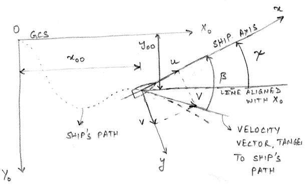
GCS and BCS frames for a three degree of freedom system is shown in Figure 3.1. Notice that velocity vector \(\vec{v} = u \hat{i} + v\hat{j}\) is tangent to the path of the ship. During a transient maneuver, the velocity vector will not point in the longitudinal direction of the ship. The angle between the velocity vector and the longitudinal direction of the ship is known as the drift angle \(\beta\). Mathematically the drift angle is defined as shown in \(\eqref{eq-drift}\).
\[\begin{align} \beta = \arctan \left(\frac{-v}{u}\right) \label{eq-drift} \end{align}\]
Surface vessels typically have port and starboard symmetry in goemetry. In order for the vessel to not have a list angle the weight in the ship is distributed such that the center of gravity lies on the centerline of the ship (\(y_G=0\)). This further means that the cross mass moments of inertia \(I_{xy}= I_{yx} = I_{yz} = I_{zy} = 0\). The maneuvering equations of motions for a surface vessel are then given by \(\eqref{eq-surge-rigid-body}\), \(\eqref{eq-sway-rigid-body}\) and \(\eqref{eq-yaw-rigid-body}\).
\[\begin{align} m\dot{u} = X \label{eq-surge-rigid-body} \end{align}\]
\[\begin{align} m \dot{v} + m x_G \dot{r} + mUr = Y \label{eq-sway-rigid-body} \end{align}\]
\[\begin{align} I_z \dot{r} + m x_G \dot{v} + m x_G U r = N \label{eq-yaw-rigid-body} \end{align}\]
\(X\), \(Y\) and \(N\) in (\(\ref{eq-surge-rigid-body}\)-\(\ref{eq-yaw-rigid-body}\)) represent the external forces and moments acting on the vessel. These can be separated into their components shown below:
- Forces and moments exerted by the fluid surrounding the vessel - denoted by \(X_F\), \(Y_F\) and \(N_F\)
- Forces and moments exerted on the body due to control surfaces like rudders, dive planes, bow planes, thrusters etc. - denoted by \(X_R\), \(Y_R\) and \(N_R\)
- Environmental forces and moments due to wind, currents and waves - denoted by \(X_E\), \(Y_E\) and \(N_E\)
- Propulsion force \(T\)
Mathematically the separation into components is shown in \(\eqref{eq-ext-force-comp}\).
\[\begin{align} X &= X_F + X_R + X_E + T \nonumber \\ Y &= Y_F + Y_R + Y_E \label{eq-ext-force-comp}\\ N &= N_F + N_R + N_E \nonumber \end{align}\]
3.1 Hydrodynamic forces and moments
The hydrodynamic forces and moments on the body \(X_F\), \(Y_F\) and \(N_F\) are caused due to the relative motion between the fluid and the structure. As shown in \(\eqref{eq-hyd-force-dependence}\) they are a function of the velocity and acceleration of the body.
\[\begin{align} X_F = X_F(\dot{u}, \dot{v}, \dot{r}, u, v, r) \nonumber \\ Y_F = Y_F(\dot{u}, \dot{v}, \dot{r}, u, v, r) \label{eq-hyd-force-dependence}\\ N_F = N_F(\dot{u}, \dot{v}, \dot{r}, u, v, r) \nonumber \end{align}\]
In general the dependence of the forces and moments on the velocities and accelerations will be strongly nonlinear. However, these nonlinear functions can be expanded as a Taylor series expansion about the nominal operating condition as described above. The Taylor series expansion upto the first order for \(Y_F\) is shown in \(\eqref{eq-hyd-force-taylor-Y}\).
\[\begin{align} Y_F (\dot{u}, \dot{v}, \dot{r}, u, v, r) =& Y_F(U,0,0,0,0,0) + \p{Y_F}{\dot{u}} (U,0,0,0,0,0) \dot{u} \nonumber \\ &+ \p{Y_F}{\dot{v}} (U,0,0,0,0,0) \dot{v} + \p{Y_F}{\dot{r}} (U,0,0,0,0,0) \dot{r} \label{eq-hyd-force-taylor-Y}\\ &+ \p{Y_F}{u} (U,0,0,0,0,0) (u - U) + \p{Y_F}{v} (U,0,0,0,0,0) v \nonumber\\ &+ \p{Y_F}{r} (U,0,0,0,0,0) r \nonumber \end{align}\]
In the nominal equilibrium condition, the vessel experiences no lateral sway force due to the symmetry of the port and starboard geometry of the vessel. The derivatives of \(Y_F\) with respect to \(\dot{u}\) and \(u\) will also be zero in the nominal condition due to symmetry. These conditions are mathematically shown in \(\eqref{eq-YF-symmetry}\).
\[\begin{align} Y_F(U,0,0,0,0,0) = \p{Y_F}{\dot{u}} (U,0,0,0,0,0) = \p{Y_F}{u} (U,0,0,0,0,0) = 0 \label{eq-YF-symmetry} \end{align}\]
Thus the Taylor expansion simplifies to \(\eqref{eq-YF-simplified}\).
\[\begin{align} Y_F (\dot{u}, \dot{v}, \dot{r}, u, v, r) = \p{Y_F}{\dot{v}} \dot{v} + \p{Y_F}{\dot{r}} \dot{r} + \p{Y_F}{v} v + \p{Y_F}{r} r \label{eq-YF-simplified} \end{align}\]
A similar expansion follows for \(X_F\) and \(N_F\) as shown in \(\eqref{eq-hyd-force-taylor-X}\) and \(\eqref{eq-hyd-force-taylor-N}\) respectively.
\[\begin{align} X_F (\dot{u}, \dot{v}, \dot{r}, u, v, r) =& X_F(U,0,0,0,0,0) \nonumber \\ &+ \p{X_F}{\dot{u}} \dot{u} + \p{X_F}{\dot{v}} \dot{v} + \p{X_F}{\dot{r}} \dot{r} \nonumber\\ &+ \p{X_F}{u} (u - U) + \p{X_F}{v} v + \p{X_F}{r} r \label{eq-hyd-force-taylor-X} \end{align}\]
\[\begin{align} N_F (\dot{u}, \dot{v}, \dot{r}, u, v, r) =& N_F(U,0,0,0,0,0) \nonumber \\ &+ \p{N_F}{\dot{u}} \dot{u} + \p{N_F}{\dot{v}} \dot{v} + \p{N_F}{\dot{r}} \dot{r} \nonumber\\ &+ \p{N_F}{u} (u - U) + \p{N_F}{v} v + \p{N_F}{r} r \label{eq-hyd-force-taylor-N} \end{align}\]
Although forward and aft symmetry does not exist for typical ships, they are slender with the breadth being significantly shorter than length. Therefore, the variation in surge force due to sway and yaw velocities and sway and yaw accelerations is negligible as shown in \(\eqref{eq-XF-symmetry}\).
\[\begin{align} \p{X_F}{\dot{v}} = \p{X_F}{\dot{r}} = \p{X_F}{v} = \p{X_F}{r} \approx 0 \label{eq-XF-symmetry} \end{align}\]
In the nominal condition, the resistance experienced by the vessel will be equal to the thrust generated by the propeller and hence \(X_F(U,0,0,0,0,0) = -T\). Thus, the Taylor expansion for \(X_F\) simplifies to \(\eqref{eq-XF-simplified}\).
\[\begin{align} X_F (\dot{u}, \dot{v}, \dot{r}, u, v, r) = -T + \p{X_F}{\dot{u}} \dot{u} + \p{X_F}{u} (u - U) \label{eq-XF-simplified} \end{align}\]
The derivatives of \(N_F\) can be simplified using similar arguments as used for the derivatives of \(Y_F\). The Taylor expansion for \(N_F\) simplifies to as shown in \(\eqref{eq-NF-simplified}\).
\[\begin{align} N_F (\dot{u}, \dot{v}, \dot{r}, u, v, r) = \p{N_F}{\dot{v}} \dot{v} + \p{N_F}{\dot{r}} \dot{r} + \p{N_F}{v} v + \p{N_F}{r} r \label{eq-NF-simplified} \end{align}\]
3.2 Control Surface Forces and Moments
For typical ships, the primary control surface is the rudder. The force experienced by the rudder is a function of the local flow characteristics near the aft of the vessel. Thus, this force would depend on the rudder angle \(\delta\), rudder rate \(\dot{\delta}\) and the velocities and accelerations of the vessel. Generally, the rudder area is about \(2\%\) of ship’s wetted surface area and hence the rudder force is much smaller when compared to the hydrodynamic forces experienced by the hull. Thus, variations in rudder force due to the ship’s motion is not a significant component in the dynamics of the vessel. Therefore, the rudder force and moment can be approximated as a function of the rudder angle alone and the Taylor expansion for the rudder force is given by \(\eqref{eq-XR-taylor}\), \(\eqref{eq-YR-taylor}\) and \(\eqref{eq-NR-taylor}\).
\[\begin{align} X_R(\delta) &= X_R(0) + \p{X_R}{\delta} \delta \label{eq-XR-taylor}\\ Y_R(\delta) &= Y_R(0) + \p{Y_R}{\delta} \delta \label{eq-YR-taylor}\\ N_R(\delta) &= N_R(0) + \p{N_R}{\delta} \delta \label{eq-NR-taylor} \end{align}\]
\(X_R(0) = \p{X_R}{\delta} \approx 0\) and thus upto leading order there is no surge force experienced due to the rudder. Note that in reality there will be drag force acting on the rudder which will be compensated by the propeller. When the rudder angle \(\delta=0\), the symmetry of the rudder and the vessel ensures that \(Y_R(0) = N_R(0) = 0\). Thus the simplified Taylor expansions for rudder forces and moment are given by \(\eqref{eq-XR-taylor-simplified}\), \(\eqref{eq-YR-taylor-simplified}\) and \(\eqref{eq-NR-taylor-simplified}\).
\[\begin{align} X_R(\delta) &= 0 \label{eq-XR-taylor-simplified}\\ Y_R(\delta) &= \p{Y_R}{\delta} \delta \label{eq-YR-taylor-simplified}\\ N_R(\delta) &= \p{N_R}{\delta} \delta \label{eq-NR-taylor-simplified} \end{align}\]
3.3 Linearized Equations in Calm Sea
The wave effects on maneuvering motions of a ship are typically neglected as wave forces have a very short time period as compared to the time scales of the transient maneuvering motions. Since ships have a significant inertia, small wind gusts too do not affect its dynamics severly. Large winds that can severely impact ships manifest during a stormy weather in the ocean. Most ships try to avoid such weather conditions by taking appropriate weather routing measures in advance. Also when a ship stuck in a storm, the focus is primarily on survivability and not on its maneuvering characteristics. Therefore, traditionally maneuvering motions have been studied primarily in calm waters.
In the recent years, new regulations are coming into affect that aim to reduce the emmission produced by ships by outfitting them with lower powered engines. When the ship has lower power, the added resistance due to the waves becomes an important parameter as the vessel should not be adrift in waves and must maintain the capability to manuever well in the waves. This has led to recent research interest in the topic of maneuvering in waves. However, for the purposes of this course, maneuvering characteristics will be studied in the traditional manner in calm seas.
In order to maintain a compact notation, the hydrodynamic derivatives are expressed with the notation shown below
\[\begin{align*} \p{X_F}{\dot{u}} &= X_{\dot{u}} \quad \p{X_f}{u} = X_u \\ \p{Y_F}{\dot{v}} &= Y_{\dot{v}} \quad \p{Y_F}{\dot{r}} = Y_{\dot{r}} \quad \p{Y_F}{v} = Y_{v} \quad \p{Y_F}{r} = Y_{r} \\ \p{N_F}{\dot{v}} &= N_{\dot{v}} \quad \p{N_F}{\dot{r}} = N_{\dot{r}} \quad \p{N_F}{v} = N_{v} \quad \p{N_F}{r} = N_{r} \end{align*}\]
Substituting \(\eqref{eq-XF-simplified}\), \(\eqref{eq-YF-simplified}\), \(\eqref{eq-NF-simplified}\), \(\eqref{eq-XR-taylor-simplified}\), \(\eqref{eq-YR-taylor-simplified}\) and \(\eqref{eq-NR-taylor-simplified}\) into \(\eqref{eq-surge-rigid-body}\), \(\eqref{eq-sway-rigid-body}\) and \(\eqref{eq-yaw-rigid-body}\) results in the linear equations of motion govering the maneuvering motions of a vessel in calm sea shown in \(\eqref{eq-surge-linear-eom}\), \(\eqref{eq-sway-linear-eom}\) and \(\eqref{eq-yaw-linear-eom}\).
\[\begin{align} (m - X_{\dot{u}}) \dot{u} = X_u (u - U) \label{eq-surge-linear-eom} \end{align}\]
\[\begin{align} (m - Y_{\dot{v}}) \dot{v} - (Y_{\dot{r}} - m x_G) \dot{r} = Y_v v + (Y_r - mU) r + Y_{\delta} \delta \label{eq-sway-linear-eom} \end{align}\]
\[\begin{align} (I_z - N_{\dot{r}}) \dot{r} - (N_{\dot{v}} - m x_G) \dot{v} = N_v v + (N_r - mx_GU) r + N_{\delta} \delta \label{eq-yaw-linear-eom} \end{align}\]
It can be seen that the surge equation is decoupled from the sway and yaw equations and is also known as the speed equation. The sway and yaw equations are coupled together and are collectively referred to as the steering equations.
It can be seen that a positive rudder angle as per right hand convention (about the rudder shaft pointing down) results in a port side rudder that turns the vessel towards the port side. Note that this convention of positive rudder angle differs from some texts that take starboard rudder as positive. However, for consistency, this text shall maintain the right hand convention along the rudder shaft as the positive rudder angle.
It is customary to non-dimensionalize the equations of motion using density \(\rho\), ship length \(L\) and design speed \(U\). The nondimensional time is defined as:
\[\begin{align*} t' = \frac{tU}{L} \end{align*}\]
Note that one unit of time is now the time it takes for the vessel to travel one ship length. The nondimensionalization of sway velocity, sway acceleration, yaw velocity and yaw acceleration is shown below:
\[\begin{align*} v' = \frac{v}{U} \quad \dot{v}' = \frac{\dot{v}L}{U^2} \quad r' = \frac{rL}{U} \quad \dot{r}' = \frac{\dot{r}L^2}{U^2} \end{align*}\]
The mass and geometric properties are non-dimensionalized as shown below:
\[\begin{align*} m' = \frac{m}{\frac{1}{2} \rho L^3} \quad I_z' = \frac{I_z}{\frac{1}{2} \rho L^5} \quad x_G' = \frac{x_G}{L} \end{align*}\]
The hydrodynamic derivatives are non-dimensionalized as shown below:
\[\begin{align*} Y_{\dot{v}}' &= \frac{Y_{\dot{v}}}{\frac{1}{2} \rho L^3} \quad Y_{\dot{r}}' = \frac{Y_{\dot{r}}}{\frac{1}{2} \rho L^4} \quad N_{\dot{v}}' = \frac{N_{\dot{v}}}{\frac{1}{2} \rho L^4} \quad N_{\dot{r}}' = \frac{N_{\dot{r}}}{\frac{1}{2} \rho L^5} \\ Y_{v}' &= \frac{Y_{v}}{\frac{1}{2} \rho L^2 U} \quad Y_{r}' = \frac{Y_{r}}{\frac{1}{2} \rho L^3 U} \quad N_{v}' = \frac{N_{v}}{\frac{1}{2} \rho L^3 U} \quad N_{r}' = \frac{N_{r}}{\frac{1}{2} \rho L^4 U} \\ Y_{\delta}' &= \frac{Y_{\delta}}{\frac{1}{2} \rho L^2 U^2} \quad N_{\delta}' = \frac{N_{\delta}}{\frac{1}{2} \rho L^3 U^2} \end{align*}\]
The non-dimensional linear equations of motion are shown in \(\eqref{eq-surge-linear-eom-nd}\), \(\eqref{eq-sway-linear-eom-nd}\) and \(\eqref{eq-yaw-linear-eom-nd}\).
\[\begin{align} (m' - X_{\dot{u}}') \dot{u}' = X_u' (u' - 1) \label{eq-surge-linear-eom-nd} \end{align}\]
\[\begin{align} (m' - Y_{\dot{v}}') \dot{v}' - (Y_{\dot{r}}' - m' x_G') \dot{r}' = Y_v' v' + (Y_r' - m') r' + Y_{\delta}' \delta \label{eq-sway-linear-eom-nd} \end{align}\]
\[\begin{align} (I_z' - N_{\dot{r}}') \dot{r}' - (N_{\dot{v}}' - m' x_G') \dot{v}' = N_v' v' + (N_r' - m'x_G') r' + N_{\delta}' \delta \label{eq-yaw-linear-eom-nd} \end{align}\]
3.4 Exercises
A ship has a length of \(100\) m and is traveling at its design speed of \(10\) m/s. If the non-dimensional time \(t' = 2\), what is the actual time in seconds that has elapsed? Explain what this time physically represents in terms of the ship’s motion.
A ship has a length of \(150\) m and is traveling at its design speed of \(10\) m/s. At a certain instant, its sway velocity is measured as \(2\) m/s and its yaw rate is \(0.02\) rad/s. Calculate:
- The non-dimensional sway velocity \(v'\)
- The non-dimensional yaw rate \(r'\)
- If the maximum allowable non-dimensional sway velocity for safe operation is \(v_{max}' = 0.3\), what is the maximum allowable actual sway velocity \(v_{max}\) in m/s?
A ship has a mass of \(5000\) tonnes and length of \(80\)m. Given that seawater density is \(1025\) kg/m³, calculate the non-dimensional mass \(m'\). What does this number physically represent?
A ship’s rudder generates a sway force of \(100\) kN at a rudder angle of \(15\) degrees when traveling at \(5\) m/s. If the ship is \(100\) m long and operates in seawater (\(\rho = 1025\) kg/m³), calculate \(Y_{\delta}'\). What would be the sway force at the same rudder angle if the speed doubled?
A ship has a non-dimensional yaw rate \(r' = 0.1\) when executing a turn. If the ship is \(150\) m long and traveling at \(12\) m/s, what is its actual yaw rate \(r\) in degrees per second?
For each of the following equations/systems, determine whether they are linear or nonlinear. Explain your reasoning.
The one-dimensional wave equation:
\(\frac{\partial^2 u}{\partial t^2} = c^2\frac{\partial^2 u}{\partial x^2}\)
The Navier-Stokes equations for incompressible flow:
\(\rho\frac{\partial \mathbf{u}}{\partial t} + \rho(\mathbf{u} \cdot \nabla)\mathbf{u} = -\nabla p + \mu\nabla^2\mathbf{u}\) \(\nabla \cdot \mathbf{u} = 0\)
The coupled system:
\(\dot{x} = 2x + y\)
\(\dot{y} = -x + 3y^2\)
The Laplace equation for potential flow:
\(\nabla^2\phi = \frac{\partial^2\phi}{\partial x^2} + \frac{\partial^2\phi}{\partial y^2} + \frac{\partial^2\phi}{\partial z^2} = 0\)
Consider the following nonlinear equation:
\(\dot{x} = -x^2 + \sin(x) + u\)
where \(u\) is a control input. Linearize this equation about the equilibrium point \(x_e = \frac{\pi}{2}\), \(u_e = 5\) using Taylor series expansion.
For each of the following coupled systems, identify:
- The coupling terms
- Whether the coupling is one-way or two-way
- The physical significance of the coupling
A mass-spring-pendulum system where a pendulum is attached to a mass that can move horizontally on a spring:
\(m_1\ddot{x} + kx = m_2l(\ddot{\theta}\cos\theta - \dot{\theta}^2\sin\theta)\)
\(m_2l^2\ddot{\theta} + m_2gl\sin\theta = -m_2l\ddot{x}\cos\theta\)
A thermal-structural system for a beam:
\(\rho c_p\frac{\partial T}{\partial t} = k\nabla^2T + \alpha E\theta_0T\frac{\partial^2w}{\partial t\partial x}\)
\(\rho A\frac{\partial^2w}{\partial t^2} + EI\frac{\partial^4w}{\partial x^4} = -\alpha E\frac{\partial^2T}{\partial x^2}\)
The roll-yaw coupling in a ship:
\(I_x\ddot{\phi} + B\dot{\phi} + C\phi = N_{\phi r}\dot{r}\)
\(I_z\ddot{r} + D\dot{r} = N_{r\phi}\dot{\phi}\)
where \(\phi\) is roll angle and \(r\) is yaw rate.
A ship has the following parameters:
- Length \(L = 120\) m
- Mass \(m = 8000\) tonnes
- Design speed \(U = 8\) m/s
- Center of gravity location \(x_G = 5\) m forward of midship
- Yaw moment of inertia \(I_z = 2.4 \times 10^8\) kg·m²
Calculate the non-dimensional parameters \(m'\), \(I_z'\), \(x_G'\) given seawater density \(\rho = 1025\) kg/m³.
Convert the following dimensional hydrodynamic derivatives to non-dimensional form given \(L = 150\) m, \(U = 10\) m/s, \(\rho = 1025\) kg/m³:
- \(Y_v = -2.5 \times 10^5\) N·s/m
- \(N_r = -8.0 \times 10^7\) N·m·s
- \(Y_{\delta} = 4.2 \times 10^5\) N
A ship is executing a steady turn with a non-dimensional yaw rate \(r' = 0.15\). Given:
- Length \(L = 180\) m
- Speed \(U = 15\) m/s
Calculate:
- The dimensional yaw rate \(r\) in rad/s
- The drift angle \(\beta\) in degreesif the non-dimensional sway velocity \(v' = -0.08\)
A ship has the following non-dimensional parameters:
\(m' = 0.022\), \(Y_v' = -0.15\), \(Y_{\dot{v}}' = -0.010\), \(Y_r' = 0.02\),
\(Y_{\dot{r}}' = -0.0005\), \(N_v' = -0.008\), \(N_{\dot{v}}' = -0.0005\), \(N_r' = -0.04\),
\(N_{\dot{r}}' = -0.002\), \(Y_{\delta}' = 0.02\), \(N_{\delta}' = -0.01\), \(I_z' = 0.002\)
At \(t' = 0\), the ship has \(v' = 0.05\) and \(r' = 0.02\). Calculate the initial non-dimensional accelerations \(\dot{v}'\) and \(\dot{r}'\) when \(\delta = 5^\circ\) (assuming no other external forces and that the BCS origin is at the center of gravity).
A ship has the following known non-dimensional parameters:
\(m' = 0.032\), \(Y_{\dot{v}}' = -0.015\), \(Y_{\dot{r}}' = 0\), \(N_{\dot{v}}' = 0\),
\(N_{\dot{r}}' = -0.0002\), \(Y_{\delta}' = 0.002\), \(N_{\delta}' = -0.002\), \(x_G' = 0.05\),
\(I_z' = 0.0002\)
Assume that the ship has a length of \(L = 200\) m, design speed of \(U = 12\) m/s and is operating in seawater with density \(\rho = 1025\) kg/m³. At \(t' = 0\), the ship has \(v' = 0.05\), \(r' = 0.02\), \(\dot{v}' = 0.01\), \(\dot{r}' = 0.004\), \(\delta = 0\). Calculate the dimensional hydrodynamic derivatives \(Y_v\) and \(N_r\) if \(N_v \approx Y_r \approx 0\).
For a ship with \(L = 100\) m and \(U = 12\) m/s, convert the following between dimensional and non-dimensional forms:
- A non-dimensional yaw acceleration \(\dot{r}' = 0.008\) to rad/s²
- A sway acceleration of \(\dot{v} = 0.05\) m/s² to \(\dot{v}'\)
A ship with \(N_{\delta}' = -0.02\) is applying a rudder of \(10^\circ\). Given:
- Length \(L = 160\) m
- Speed \(U = 8\) m/s
- \(\rho = 1025\) kg/m³
Calculate:
- The dimensional yaw moment \(N_{\delta}\) in kN·m
- The yaw moment in kN·m at the same rudder angle if speed increases to \(12\) m/s
- The required rudder angle to maintain the same yaw moment at \(12\) m/s
Answer Key
The actual time in seconds that has elapsed is \(20.0\) seconds.
This means that the ship has traveled \(2\) ship lengths (\(200.0\) meters) at its design speed of \(10\) m/s.
The non-dimensional sway velocity is \(v' = 0.20\)
The non-dimensional yaw rate is \(r' = 0.30\)
The maximum allowable actual sway velocity is \(v_{max} = 3.00\) m/s
The non-dimensional mass is \(m' = 0.019055\)
This represents the ratio of ship’s mass to the half the mass of water in a volume proportional to ship’s length cubed.
\(Y_\delta' = 0.000780\)
At double speed (\(10\) m/s), the force would be \(400.0\) kN (\(4.0\) times) due to the \(U^2\) term in the denominator of the non-dimensionalization.
The actual yaw rate is \(r = 0.46\) degrees/s
Linearity Analysis:
The wave equation is linear because:
All terms involve the dependent variable u or its derivatives to the first power
The coefficients (c²) are constants
The principle of superposition applies
The Navier-Stokes equations are nonlinear because:
The convective acceleration term \(\rho(\mathbf{u} \cdot \nabla)\mathbf{u}\) contains products of the velocity components
This nonlinear term makes the equations very difficult to solve analytically
This system is nonlinear because:
While the first equation is linear (only first power terms in \(x\) and \(y\))
The second equation contains \(y^2\), which is nonlinear
The principle of superposition does not apply to this system
The Laplace equation is linear because:
All terms are second derivatives of \(\phi\) to the first power
The coefficients are constants (1)
The principle of superposition applies - if \(\phi_1\) and \(\phi_2\) are solutions, then \(a\phi_1 + b\phi_2\) is also a solution for any constants \(a\) and \(b\)
The linearized equation is given by:
\(\dot{x} = 3.47 -3.14x + 1.00u\)
Analysis of coupled systems:
- Mass-spring-pendulum system:
- Coupling terms: \(m_2l(\ddot{\theta}\cos{\theta} - \dot{\theta}^2\sin{\theta})\) in first equation and \(-m_2l\ddot{x}\cos{\theta}\) in second equation
- Two-way coupling: The motion of mass affects pendulum and vice versa
- Physical significance: Represents inertial coupling between horizontal motion and pendulum swing
- Thermal-structural system:
- Two-way coupling: Temperature affects displacement and displacement rate affects temperature
- Physical significance: Represents thermoelastic coupling where deformation causes heating and temperature gradients cause stress
- Roll-yaw coupling:
- Coupling terms: \(N_{\phi r}\dot{r}\) in roll equation and \(N_{r\phi}\dot{\phi}\) in yaw equation
- Two-way coupling: Roll rate affects yaw motion and yaw rate affects roll motion
- Physical significance: Represents gyroscopic coupling between roll and yaw motions in ships, particularly important in high-speed vessels
- Mass-spring-pendulum system:
The non-dimensional parameters are:
\(m' = 0.009033\)
\(I_z' = 0.000019\)
\(x_G' = 0.041667\)
The non-dimensional parameters are:
\(Y_v' = -0.002168\)
\(N_r' = -0.000031\)
\(Y_{\delta}' = 0.000364\)
The dimensional yaw rate is \(r = 0.0125\) rad/s
The drift angle is \(\beta = 4.59\) degrees
The initial non-dimensional accelerations are \(\dot{v}' = -0.173326\) and \(\dot{r}' = -0.496500\)
The dimensional hydrodynamic derivatives are:
\(Y_v = 5.492688 \times 10^6\) N·s/m
\(N_r = 24403.20 \times 10^6\) N·m·s
The dimensional yaw acceleration is \(\dot{r} = 0.000115\) rad/s²
The dimensional sway acceleration is \(\dot{v} = 0.034722\) m/s²
The dimensional yaw moment is \(N_{\delta} = -468965.78\) kN·m
The yaw moment at \(U = 12\) m/s is \(N_{\delta} = -1055173.01\) kN·m
The required rudder angle to maintain the same yaw moment at \(U = 12\) m/s is \(\delta = 4.44\) degrees