8 Estimting Hydrodynamic Coefficients
The previous chapters described the linearized as well as the nonlinear maneuvering equations of motion for a ship. In order to ascertain the stability or to even simulate the motions of a vessel in the ocean, the hydrodynamic derivatives and coefficients must be known. This chapter will focus on the estimation of hydrodynamic derivatives and hydrodynamic coefficients using experimental, theoretical and empirical approaches. During the basic design phase the theoretical and empirical approaches are preferred and during the later design stage experimental methods are preferred to ascertain the maneuvering characteristics of the design.
8.1 Theoretical Methods to Evaluate Hydrodynamic Derivatives
The theoretical computation of hydrodynamic derivatives has been a challenging problem for a long time. With the advancement of computational power, there is considerable interest in using computational fluid dynamics (CFD) to predict the hydrodynamic derivatives. Even with the currently available computational resources, it is significantly challenging to predict the hydrodynamic derivatives of full scale ships as the flow past a ship is highly turbulent with \(Re \sim \mathcal{O}\left(10^9\right)\). This process is quite time consuming and hence not quite suitable for a design process.
Some success has been achieved through the use of potential flow methods. These are largely relevant in evaluating the acceleration hydrodynamic derivatives (\(X_{\dot{u}}\), \(Y_{\dot{v}}\), \(Y_{\dot{r}}\), \(N_{\dot{v}}\) and \(N_{\dot{r}}\)) that represent the added mass of the vessel. Their evaluation at zero frequency, corresponding to the assumption of slow motion, is now a fairly accepted method of estimation. However, the hydrodynamic damping derivatives (\(X_u\), \(Y_v\), \(Y_r\), \(N_v\) and \(N_r\)) encode the viscous effects and cannot be effectively evaluated by potential theory.
Some of the early attempts to predict the hydrodynamic derivatives relied on modelling the ship as a slender body and assume it to behave like a low aspect ratio aerofoil. Applying finite span aerofoil theory, it can be shown that the hydrodynamic damping derivatives are given by
\[\begin{align} Y_{v}' &= -\pi\left(\frac{T}{L}\right)^2 \times (1) \\ Y_{r}' &= -\pi\left(\frac{T}{L}\right)^2 \times \left(-\frac{1}{2}\right) \\ N_{v}' &= -\pi\left(\frac{T}{L}\right)^2 \times \left(\frac{1}{2}\right) \\ N_{r}' &= -\pi\left(\frac{T}{L}\right)^2 \times \left(\frac{1}{4}\right) \end{align}\]
The viscosity effects near the stern of a ship are dominant and the flow is a complex function of the geometry. The complexity of the flow makes the applicability of the above expressions very limited and not practical.
The rudder hydrodynamic derivatives (\(Y_{\delta}\), \(N_{\delta}\), \(X_{\delta \delta}\) and others) can be evaluated using existing lift and drag coefficient data for standard aerofoil sections.
8.2 Empirical Methods to Evaluate Hydrodynamic Derivatives
The direct theoretical evaluation of damping hydrodynamic derivatives is still considered to be not very practical. This has given rise to the semi-empirical approaches that aim to use regression techniques to combine data from several ships to yeild formulations for damping and acceleration hydrodynamic derivatives as a function of principal dimensions. Some of these expressions summarized from PNA (Principles of Naval Architecture) Vol III are shown below.
\[\begin{align} Y_{\dot{v}}' &= -\pi\left(\frac{T}{L}\right)^2 \times \left[1 + 0.16 C_B \frac{B}{T} - 5.1 \left(\frac{B}{L}\right)^2\right] \\ Y_{\dot{r}}' &= -\pi\left(\frac{T}{L}\right)^2 \times \left[0.67 \frac{B}{L} - 0.0033 \left(\frac{B}{T}\right)^2\right] \\ N_{\dot{v}}' &= -\pi\left(\frac{T}{L}\right)^2 \times \left[1.1\frac{B}{L} - 0.041 \frac{B}{T}\right] \\ N_{\dot{r}}' &= -\pi\left(\frac{T}{L}\right)^2 \times \left[\frac{1}{12} + 0.017 C_B \frac{B}{T} - 0.33 \frac{B}{L}\right] \\ Y_{v}' &= -\pi\left(\frac{T}{L}\right)^2 \times \left[1 + 0.4C_B \frac{B}{T}\right] \\ Y_{r}' &= -\pi\left(\frac{T}{L}\right)^2 \times \left[-\frac{1}{2} + 2.2\frac{B}{L} - 0.08 \frac{B}{T}\right] \\ N_{v}' &= -\pi\left(\frac{T}{L}\right)^2 \times \left[\frac{1}{2} + 2.4\frac{T}{L}\right] \\ N_{r}' &= -\pi\left(\frac{T}{L}\right)^2 \times \left[\frac{1}{4} + 0.039\frac{B}{T} - 0.56 \frac{B}{L}\right] \end{align}\]
It is important to note that empirical formulas as above have limited statistical significance and must be used with caution, especially when exploring newer designs that have significant variations from known designs or designs used for regressing the empirical formulas.
8.3 Experimental Model Tests
The primary approach to estimate the maneuvering hydrodynamic coefficients is to conduct controlled experiments with scaled models of the real ship. This is adopted fairly late in the design process where the hull linesplan is being finalized. The objective of these experiments is to ascertain the hydrodynamic derivatives through captive model tests where the model is moved through water in captive manner and the forces acting on the body are measured through load cells. The common model tests performed include:
- Straight line tests
- Rotating arm tests
- Planar motion mechanism (PMM) tests
- Free running model tests (gaining traction recently)
8.3.1 Straight Line Test
A model geometrically similar to the propotype is created and towed in the towing tank as shown in Figure 8.1. The towing speed is decided by matching the Froude number between the model and the prototype.
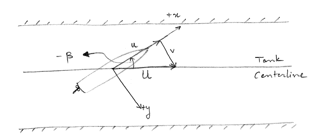
The model is rigidly fixed to a carriage through a dynamometer. The carriage moves across the length of the tank with a speed \(U\). Several runs are conducted at different drift angles \(\beta\). In each test, the dynamometer measures the sway force \(Y\) and yaw moment \(N\) acting on the vessel. A specific \(\beta\) results in a sway velocity given by
\[\begin{align} v = -U \sin(\beta) \end{align}\]
Collecting all the data, a plot of \(Y\) vs \(v\) and a plot of \(N\) vs \(v\) is generated. The slope of this curve at \(v=0\) yields \(Y_v\) and \(N_v\). The nonlinear coefficients like \(Y_{vvv}\) can also be obtained by curve fitting the data. The obtained coefficients are non-dimensionalized based on model dimension and speed. The non-dimensional coefficients can now be used for the actual vessel in full scale.
Note that scale effects are encountered in this approach as the Reynolds number is not the same between the model and prototype. In general, it is not possible to achieve Reynolds similarity between the model and prototype as the required velocities cannot be achieved in a practical towing experiment.
Since the propeller affects the hydrodynamic derivatives and coefficients, sometimes the model is affixed with the propeller and is operated at the self propulsion point. The straight line tests can also be used to evaluate the ruder hydrodynamic derivatives such as \(Y_{\delta}\) and \(N_{\delta}\). In this case the model is towed with zero drift angle (\(\beta=0\)) but with different rudder deflections \(\delta\).
8.3.2 Rotating Arm Test
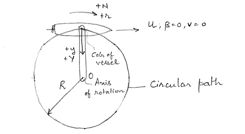
The straight line test generated a pure sway condition by towing the model with a drift angle. Thus it can be used to evaluate the sway hydrodynamic derivatives \(Y_v\) and \(N_v\). In order to evaluate the yaw hydrodynamic derivatives \(Y_r\) and \(N_r\), a pure yaw condition is required. This is achieved through the rotating arm test.
The model of the vessel is attached to an arm in a water basin as seen in Figure 8.2. The arm revolves about the axis of rotation \(O\) with a fixed yaw rate \(r\). Note that the vessel in this case is purely yawing with \(v=0\). Several tests are conducted by varying the value of \(r\) while maintaining the same forward speed \(U\). This is achieved by adjusting the radial distance to the attachment point along the arm denoted by \(R = \frac{U}{r}\). The dynamometer measures the sway force \(Y\) and yaw moment \(N\) across the various tests. The slopes of the \(Y\) vs \(r\) and \(N\) vs \(r\) plots at \(r=0\) yield \(Y_r\) and \(N_r\). The nonlinear hydrodynamic coefficients can be obtained by curve-fitting.
There are two limitations of the rotating arm test:
Measurements must be performed within a single revolution of the arm as otherwise the vessel will be in its own wake and will no longer represent the calm water condition.
Accurate estimation of \(Y_r\) and \(N_r\) requires measurements to be performed at small \(r\) values. This implies a large value of \(R\) as \(U\) is fixed. Thus, rotating arms require considerable space and are very expensive facilities to construct.
8.3.3 Planar Motion Mechanism (PMM) Test
PMM tests were developed to avoid the large costs associated with a rotating arm facility. The primary idea is to superimpose a transverse (sway) motion or a rotational (yaw) motion with a straight line motion and enable these tests to be conducted in the towing tank. The model of the vessel is attached to the towing tank carriage through two oscillators. One is connected to the model near its bow and another near its stern region. By adjusting the phase difference between the oscillators, a sinusoidal sway or a sinusoidal yaw can be introduced independently. The PMM setup described above is shown in Figure 8.3.
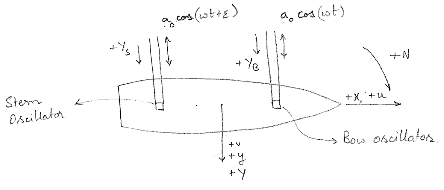
The carriage along with the model move along the length of the towing tank at a constant speed \(U\). The transducers at the oscillators measure the forces \(Y_S\) and \(Y_B\) denoting the lateral forces on stern and bow oscillators respectively. The resulting sway force \(Y\) and yaw moment \(N\) are given by
\[\begin{align} Y = Y_S + Y_B \\ N = Y_S l_S + Y_B l_B \end{align}\]
where \(l_S\) and \(l_B\) denote the lever arms of the stern and bow oscillators from the BCS origin \(O\). The lever arm is measured from the BCS origin and is considered positive along the x-axis of the ship.
Pure Sway Test
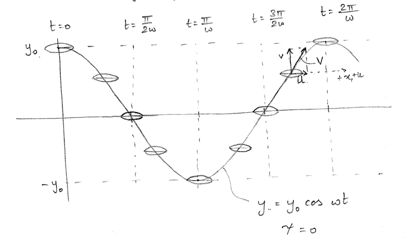
Assuming that the sinusoidal motion is given by \(\eqref{eq-pure-sway-motion}\) and as shown in Figure 8.4.
\[\begin{align} y = y_0 \cos(\omega t) \label{eq-pure-sway-motion} \end{align}\]
The sway velocity is given by \(v = \dot{y} = -y_0 \omega \sin(\omega t)\). The resulting hydrodynamic force in sway is given by
\[\begin{align} Y &= Y_v v + Y_{\dot{v}} \dot{v} + Y_{\ddot{v}} \ddot{v} + ... \\ &= (Y_v - \omega^2 Y_{\ddot{v}} + ...)(-y_0 \omega \sin(\omega t)) \nonumber \\ &\quad + (Y_{\dot{v}} - \omega^2 Y_{\dddot{v}} + ...)(-y_0 \omega^2 \cos(\omega t)) \\ &= \tilde{Y}_{v} v + \tilde{Y}_{\dot{v}} \dot{v} \end{align}\]
\(\tilde{Y}_{v} v\) represents the component of the total force at \(90^{\circ}\) phase difference with motion \(y\). \(\tilde{Y}_{\dot{v}} \dot{v}\) represents the component of the total force in phase or out of phase (\(0^{\circ}\) or \(180^{\circ}\) phase difference) with \(y\). The measurement \(Y\) includes both the components together. Each component can be separated utilizing the orthogonality of sine and cosine signals (Fourier series analysis) as shown below.
\[\begin{align} \tilde{Y}_{v} &= \frac{-1}{y_0 \omega} \left[\frac{\omega}{\pi} \int_{\frac{-\pi}{\omega}}^{\frac{\pi}{\omega}} Y \sin(\omega t) dt\right] = \frac{-1}{y_0\pi}\left[\int_{\frac{-\pi}{\omega}}^{\frac{\pi}{\omega}} Y \sin(\omega t) dt\right]\\ \tilde{Y}_{\dot{v}} &= \frac{-1}{y_0 \omega^2} \left[\frac{\omega}{\pi} \int_{\frac{-\pi}{\omega}}^{\frac{\pi}{\omega}} Y \cos(\omega t) dt\right] = \frac{-1}{y_0\omega\pi}\left[\int_{\frac{-\pi}{\omega}}^{\frac{\pi}{\omega}} Y \cos(\omega t) dt\right] \end{align}\]
In the limit \(\omega \rightarrow 0\),
\[\begin{align} \lim_{\omega \rightarrow 0} \tilde{Y}_{v} = Y_v \\ \lim_{\omega \rightarrow 0} \tilde{Y}_{\dot{v}} = Y_{\dot{v}} \end{align}\]
\(N_v\) and \(N_{\dot{v}}\) can be evaluated in a similar manner by separating the total moment \(N\) along its in phase component and its \(90^{\circ}\) out of phase components.
Pure Yaw Test
Similar to the pure sway condition, the pure yaw condition in a PMM test is obtained by superimposing a pure yaw motion with a straight line motion. In order to produce a pure yaw motion, the oscillators will still need to have a sinusoidal motion but with an appropriate phase difference. Let us assume that the stern and bow oscillators move as described in \(\eqref{eq-stern-oscillator-motion}\) and \(\eqref{eq-bow-oscillator-motion}\) respectively.
\[\begin{align} y_S = y_0 \sin(\omega t + \epsilon_S) \label{eq-stern-oscillator-motion} \\ y_B = y_0 \sin(\omega t + \epsilon_B) \label{eq-bow-oscillator-motion} \end{align}\]
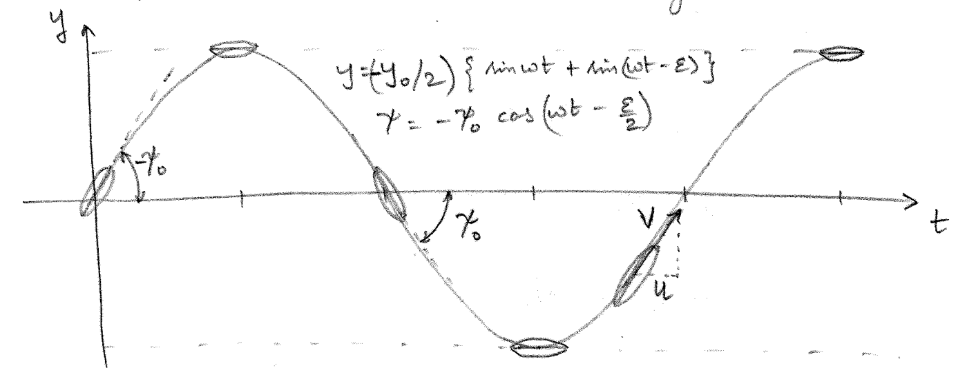
During a pure yaw motion as depicted in Figure 8.5 the motion \(y(t)\) of the model lateral to the tank will be described by
\[\begin{align} y(t) &= y_0 \sin(\omega t) \end{align}\]
The motion \(y(t)\) is obtained by the linear combination of the oscillators and can be expressed as shown below
\[\begin{align} y &= y_0 \sin(\omega t) \label{eq-pure-yaw-lat-motion-1}\\ &= y_S \frac{l_B}{l_B - l_S} + y_B \frac{-l_S}{l_B - l_S} \\ &= \frac{y_0}{l_B - l_S} \left[l_B \sin(\omega t + \epsilon_S) - l_S \sin(\omega t + \epsilon_B)\right] \\ &= \frac{y_0}{l_B - l_S} \left[l_B \cos(\epsilon_S) - l_S \cos(\epsilon_B)\right] \sin(\omega t) \nonumber \\ &\qquad + \frac{y_0}{l_B - l_S} \left[l_B \sin(\epsilon_S) - l_S \sin(\epsilon_B)\right] \cos(\omega t) \label{eq-pure-yaw-lat-motion-2} \end{align}\]
By comparing the coefficients of \(\sin(\omega t)\) and \(\cos(\omega t)\) in \(\eqref{eq-pure-yaw-lat-motion-1}\) and \(\eqref{eq-pure-yaw-lat-motion-2}\) the following two equations are obtained.
\[\begin{align} \cos(\epsilon_S) &= \cos(\epsilon_B) \approx 1 \label{eq-assumption-1}\\ l_B \sin(\epsilon_S) &= l_S \sin(\epsilon_B) \label{eq-assumption-2} \end{align}\]
The heading angle at any instant is given by
\[\begin{align} \tan(\psi) &= \frac{y_B - y_S}{l_B - l_S} \\ &= \frac{y_0}{l_B - l_S} (\cos(\epsilon_B) - \cos(\epsilon_S)) \sin(\omega t) \nonumber \\ & \qquad + \frac{y_0}{l_B - l_S} (\sin(\epsilon_B) - \sin(\epsilon_S)) \cos(\omega t) \end{align}\]
Using \(\eqref{eq-assumption-1}\) and \(\eqref{eq-assumption-2}\), the heading angle expression simplifies to
\[\begin{align} \tan(\psi) &= \frac{y_0}{l_B - l_S} \left(1 - \frac{l_S}{l_B}\right) \sin(\epsilon_B) \cos(\omega t) \\ &= \frac{y_0}{l_B} \sin(\epsilon_B) \cos(\omega t) \label{eq-heading-1} \end{align}\]
The instantaneous velocity of the model in the lateral direction to the tank is given by
\[\begin{align} \dot{y} &= \omega y_0 \cos(\omega t) \end{align}\]
In a pure yaw condition, the instantaneous direction of the velocity vector must coincide with the instantaneous longitudinal direction of the model. Mathematically this is denoted by
\[\begin{align} \tan(\psi) = \frac{\dot{y}}{U} = \frac{\omega y_0}{U} \cos(\omega t) \label{eq-heading-2} \end{align}\]
Comparing \(\eqref{eq-heading-1}\) and \(\eqref{eq-heading-2}\) and utilizing \(\eqref{eq-assumption-2}\) yields the required phase angles \(\epsilon_B\) and \(\epsilon_S\) to achieve a pure yaw maneuver as shown below.
\[\begin{align} \epsilon_B &= \sin^{-1}\left(\frac{\omega l_B}{U} \right)\\ \epsilon_S &= \sin^{-1}\left(\frac{\omega l_S}{U} \right) \end{align}\]
Assuming that the heading angle \(\psi\) is small \((\psi \approx \tan(\psi))\), the yaw rate \(r\) is given by
\[\begin{align} r = \dot{\psi} \approx - \frac{\omega^2 y_0}{U} \sin(\omega t) \end{align}\]
The resulting hydrodynamic moment in yaw is given by
\[\begin{align} N &= N_r r + N_{\dot{r}} \dot{r} + N_{\ddot{r}} \ddot{r} + ... \\ &= (N_r - \omega^2 N_{\ddot{r}} + ...)\left(- \frac{\omega^2 y_0}{U} \sin(\omega t)\right) \nonumber \\ &\quad + (N_{\dot{r}} - \omega^2 N_{\dddot{r}} + ...)\left(- \frac{\omega^3 y_0}{U} \cos(\omega t)\right) \\ &= \tilde{N}_{r} r + \tilde{N}_{\dot{r}} \dot{r} \end{align}\]
\(\tilde{N}_{r} r\) represents the component of the total moment in phase with the yaw rate \(r\). \(\tilde{N}_{\dot{r}} \dot{r}\) represents the component of the total moment that is \(90^{\circ}\) out of phase with \(r\). The measurement \(N\) includes both the components together. Each component can be separated utilizing the orthogonality of sine and cosine signals (Fourier series analysis) as shown below.
\[\begin{align} \tilde{N}_{r} &= \frac{-U}{y_0 \omega^2} \left[\frac{\omega}{\pi} \int_{\frac{-\pi}{\omega}}^{\frac{\pi}{\omega}} N \sin(\omega t) dt\right] = \frac{-U}{y_0\omega\pi}\left[\int_{\frac{-\pi}{\omega}}^{\frac{\pi}{\omega}} N \sin(\omega t) dt\right]\\ \tilde{N}_{\dot{r}} &= \frac{-U}{y_0 \omega^3} \left[\frac{\omega}{\pi} \int_{\frac{-\pi}{\omega}}^{\frac{\pi}{\omega}} N \cos(\omega t) dt\right] = \frac{-U}{y_0\omega^2\pi}\left[\int_{\frac{-\pi}{\omega}}^{\frac{\pi}{\omega}} N \cos(\omega t) dt\right] \end{align}\]
In the limit \(\omega \rightarrow 0\),
\[\begin{align} \lim_{\omega \rightarrow 0} \tilde{N}_{r} = N_r \\ \lim_{\omega \rightarrow 0} \tilde{N}_{\dot{r}} = N_{\dot{r}} \end{align}\]
\(Y_r\) and \(Y_{\dot{r}}\) can be evaluated in a similar manner by separating the total force \(Y\) along its in phase component and its \(90^{\circ}\) out of phase components.
8.3.4 Free Running Model Tests
In this test a radio controlled free running model is subjected to various maneuvers with a prescribed input (rudder angle and propeller rate input commands). Unlike in the captive model tests described above, the forces cannot be measured in a free running experiment. Rather the motions of the vessel can be measured by equipping the vessel with inertial measurement unit (IMU) and a positioning sensor such as GPS or visual positioning system. Knowing the input and outputs of the system, the hydrodynamic coefficients can be estimated through a system identification exercise. The coefficients are tuned such that the predicted motions of the system (using the hydrodynamic coefficients predicted by system identification) agree closely with real motion data captured from the experiments. More information on recommended procedures and guideline by International Towing Tank Conference (ITTC) on the conduct of free running model experiments can be found here.
8.4 Exercises
For a ship with \(L=120\) m and \(T=8\) m, compute \(\left(T/L\right)\) and \(\pi\left(T/L\right)^2\).
In a straight-line test at \(U=1.6\) m/s and \(\beta=5^\circ\), compute sway velocity.
In pure yaw PMM, let \(U=1.0\) m/s, \(\omega=0.4\) rad/s, \(l_B=1.2\) m, \(l_S=-1.2\) m. Compute \(\epsilon_B\) and \(\epsilon_S\).
For two candidate derivatives, Case A: \(Y_v=-60\) N·s/m and Case B: \(Y_v=+60\) N·s/m, compute the force \(Y=Y_v v\) for \(v=+0.2\) m/s and state which case shows a damping behavior and explain why.
In a PMM identification, two tests give \(\tilde{Y}_v'=-0.020\) at \(\omega=0.8\) rad/s and \(\tilde{Y}_v'=-0.016\) at \(\omega=0.2\) rad/s. State which estimate should be preferred and why.
A slender-body estimate gives \(Y_v'=-0.0112\) while an empirical estimate gives \(Y_v'=-0.0179\). Compute the percentage increase in magnitude from slender-body to empirical and state one physical reason for this increase.
Using the empirical formula in this chapter, compute \(Y_{\dot v}'\) for \(L=160\) m, \(B=26\) m, \(T=10\) m, \(C_B=0.62\).
Compute the four empirical damping derivatives \(Y_v'\), \(Y_r'\), \(N_v'\), and \(N_r'\) for \(L=180\) m, \(B=30\) m, \(T=11\) m, \(C_B=0.64\).
A straight-line test at \(U=1.5\) m/s gives:
| Beta (deg) | Y (N) |
|---|---|
| 2 | 3.2 |
| 4 | 6.4 |
| 6 | 9.9 |
| 8 | 13.3 |
| 10 | 16.9 |
Compute \(Y_v\) using least squares fit through this data.
For \(L=200\) m, \(B=32\) m, \(T=12\) m, \(C_B=0.58\), compute:
- Slender-body \(Y_v',Y_r',N_v',N_r'\).
- Empirical \(Y_v',Y_r',N_v',N_r'\).
- The stability index \(C'\) for both models assuming \(x_G'=0\).Compare the two \(C'\) values.
In a PMM pure sway test, assume \(Y(t)=-24\sin(\omega t)-12\cos(\omega t)\ \text{N}\) with \(y_0=0.25\) m and \(\omega=0.6\) rad/s. Compute \(\tilde{Y}_v\) and \(\tilde{Y}_{\dot v}\).
Programming problem: Write a Python script that takes a list of hull forms \((L,B,T,C_B)\) and computes all eight empirical derivatives from this chapter. Run it for:
- Hull A: \((150,24,9,0.60)\)
- Hull B: \((150,30,9,0.68)\)
- Hull C: \((150,36,8,0.82)\)
Rank the hulls by \(|Y_v'|\) and comment on sign consistency.
Three test plans are compared using weighted score: [ S=0.4Q+0.35C+0.25P ] where \(Q\) is derivative coverage score, \(C\) is confidence score, and \(P\) is practicality score (all out of 10).
Plan A (Straight-line): \((Q,C,P)=(4,6,9)\)
Plan B (Rotating arm): \((5,7,4)\)
Plan C (PMM): \((9,8,7)\)
Compute \(S\) for each and choose the plan.A model test gives \(Y_v'=-0.018\) at model scale. For a prototype with \(L=180\) m and service speed \(U=20\) knots, estimate full-scale dimensional \(Y_v\) using [ Y_v=Y_v’(L2U), 3. ] Convert \(U\) to m/s and report \(Y_v\).
Programming problem: For straight-line data at \(U=1.4\) m/s, [ (^,Y )=(0,0),(4,5.1),(8,10.8),(12,17.9),(16,28.7),(20,44.1), ] fit: [ Y=Y_vv,Y=Y_vv+Y_{vvv}v^3,v=-U ] and compute RMSE for both models. Choose the better model and interpret the result.
Answer Key
\((T/L) = 0.0667, ~\pi(T/L)^2 = 0.01396\)
\(v = -0.1394 ~m/s\)
\(\epsilon_B = 28.69^{\circ} ,~ \epsilon_S = -28.69^{\circ}\)
Case A: \(Y = -12.00 ~N\), Case B: \(Y = 12.00 ~N\)
Damping behavior: Case A. The force opposes the velocity and will eventually damp out the motion
The estimate from lower-frequency value (\(\omega = 0.2 ~rad/s\)) should be preferred as the higher order derivatives will show a greater contribution at higher frequencies.
Magnitude increase = \(59.82 \%\)
Reason: empirical relation includes viscous/geometry effects beyond slender-body assumptions.
\(Y_\dot{v}' = -0.01378\)
\(Y_v' = -0.01992\)
\(Y_r' = 0.00412\)
\(N_v' = -0.00759\)
\(N_r' = -0.00309\)
Least-squares \(Y_v = -63.91 ~N.s/m\)
Slender-body: \(Y_v'=-0.01131, Y_r'=0.00565, N_v'=-0.00565, N_r'=-0.00283, C=9.82 \times 10^{-7}\)
Empirical: \(Y_v'=-0.01831, Y_r'=0.00409, N_v'=-0.00728, N_r'=-0.00299, C=33.98 \times 10^{-7}\)
Higher \(C\) here: empirical model
\(\tilde{Y}_v = 160.00 ~N.s/m, \tilde{Y}_{\dot{v}} = 133.33 ~kg\)
Empirical derivatives for hulls:
Hull A: \(Y_v'=-0.01855, Y_r'=0.00409, N_v'=-0.00728, N_r'=-0.00299\)
Hull B: \(Y_v'=-0.02156, Y_r'=0.00369, N_v'=-0.00728, N_r'=-0.00303\)
Hull C: \(Y_v'=-0.02213, Y_r'=0.00297, N_v'=-0.00561, N_r'=-0.00260\)
Rank by |\(Y_v'\)|: C > B > A
S_A = 5.95, S_B = 5.45, S_C = 8.15 Best plan: C (PMM)
U = 10.288 m/s, Y_v = -3.07e+06 N.s/m
Linear: Y_v = -78.38, RMSE = 4.005 N Cubic : Y_v = -45.58, Y_vvv = -200.56, RMSE = 0.351 N Better model: cubic (captures nonlinearity at larger drift angles).