18 Tutorial 06 - Nomoto Models

Question 01

The yaw rate of a ship in a control fixed scenario (\(\delta = 0^{\circ}\)) changes from \(0.01 ~ rad/s\) to \(0.005 ~rad/s\) over \(4~s\) time. Estimate the time constant of the ship.

Question 02

A ship has the following non-dimensional parameters: \(m' = 0.2\), \(x_G' = 0.1\), \(Y_v' = -0.4\), \(Y_r' = 0.15\), \(N_v' = -0.05\), \(N_r' = -0.1\), \(Y_\delta' = 0.3\). Calculate the turning radius \(R\) for a rudder angle \(\delta = 5^{\circ}\) if the length of the ship is \(L = 100\) m.

Question 03

Consider a ship of length \(L=150~m\) and a design speed of \(U=12~knots\) with \(K'=-1\) and \(T'=2\). For an applied constant rudder of \(\delta = 20^{\circ}\), determine:

The radius of the turn in meters
Time for the yaw rate to reach \(63.2 \%\) of the steady value in the turn from the nominal operating condition. Compare it with the Nomoto time constant of the ship.

Question 04

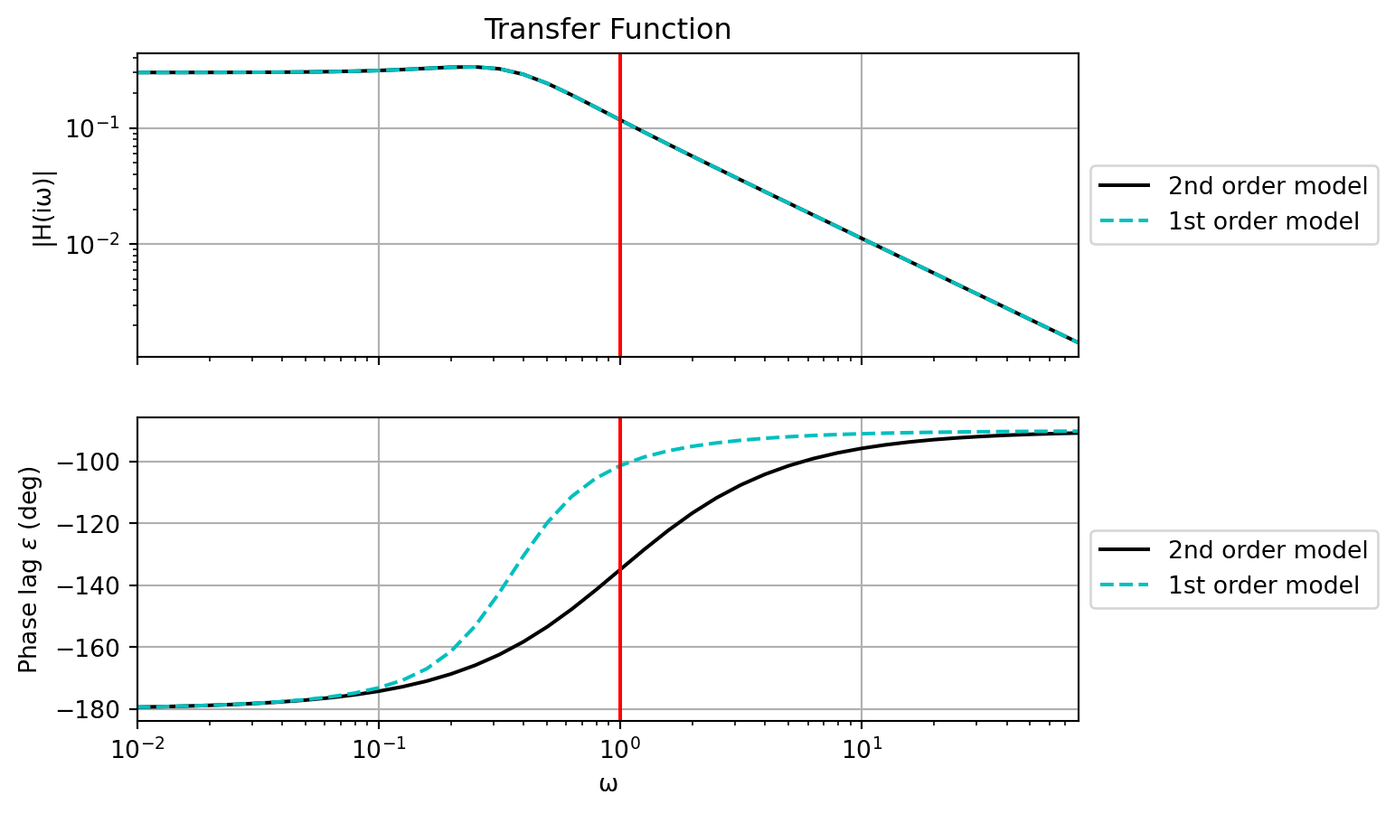
Consider a second-order Nomoto model that has the following transfer function:

\[\begin{align} \frac{r_0}{\delta_0} = -\left(\frac{0.3 + 0.9s}{1 + 4s + 8s^2}\right) \nonumber \end{align}\]

Locate the poles of the transfer function and comment on the stability of the system
Determine the time constants of the system
Write down the equivalent first-order transfer function
Cut-off frequency for a system is defined as the frequency at which the amplitude ratio is \(\frac{1}{\sqrt{2}}\) of the steady-state value (value at \(\omega = 0\)). Determine the cut-off frequency for the first-order model. Calculate the phase lag for first-order and second-order system at this frequency and compare them.

Question 01 Solution

The yaw rate of a ship in a control fixed scenario (\(\delta = 0^{\circ}\)) changes from \(0.01 ~ rad/s\) to \(0.005 ~rad/s\) over \(4~s\) time. Estimate the time constant of the ship.

Code

import numpy as np

def solve_problem_1():
    t = 4
    rt = 0.005
    r0 = 0.01
    T = t / (np.log(r0) - np.log(rt))
    
    print(f"The time constant is {T:.2f} seconds")
    
solve_problem_1()

The time constant is 5.77 seconds

Question 02 Solution

Code

import numpy as np

def solve_problem_2(): 
    L = 100
    m_prime = 0.2
    x_G_prime = 0.1
    Y_v_prime = -0.4
    Y_r_prime = 0.15
    N_v_prime = -0.05
    N_r_prime = -0.1
    Y_delta_prime = 0.3
    
    K_prime = (N_v_prime * Y_delta_prime - Y_v_prime * Y_delta_prime) / ((N_r_prime - m_prime * x_G_prime) * Y_v_prime - (Y_r_prime - m_prime) * N_v_prime)
    
    delta = 5 * np.pi / 180
    R = L / (K_prime * delta)
    
    print(f"The turning radius is {R:.2f} m\n")
    
solve_problem_2()

The turning radius is 496.56 m

Question 03 Solution

Consider a ship of length \(L=150~m\) and a design speed of \(U=12~knots\) with \(K'=-1\) and \(T'=2\). For an applied constant rudder of \(\delta = 20^{\circ}\), determine:

The radius of the turn in meters
Time for the yaw rate to reach \(63.2 \%\) of the steady value in the turn from the nominal operating condition. Compare it with the Nomoto time constant of the ship.

Code

import numpy as np

def solve_problem_3():
    L = 150
    U = 12 * 0.514444
    Kp = -1
    Tp = 2
    K = Kp * U / L
    T = Tp * L / U
    
    delta = 20 * np.pi / 180
    
    R = U / np.abs(K * delta)
    t = -T * np.log(1 - 0.632)
    
    print(f"The radius of the turn is {R:.2f} m")
    print(f"The time for the yaw rate to reach 63.2% of the steady value is {t:.2f} seconds")

solve_problem_3()

The radius of the turn is 429.72 m
The time for the yaw rate to reach 63.2% of the steady value is 48.58 seconds

Question 04 Solution

Consider a second-order Nomoto model that has the following transfer function:

\[\begin{align} \frac{r_0}{\delta_0} = -\left(\frac{0.3 + 0.9s}{1 + 4s + 8s^2}\right) \nonumber \end{align}\]

Locate the poles of the transfer function and comment on the stability of the system
Determine the time constants of the system
Write down the equivalent first-order transfer function
Cut-off frequency for a system is defined as the frequency at which the amplitude ratio is \(\frac{1}{\sqrt{2}}\) of the steady-state value (value at \(\omega = 0\)). Determine the cut-off frequency for the first-order model. Calculate the phase lag for first-order and second-order system at this frequency and compare them.

Code

import numpy as np
import matplotlib.pyplot as plt

def solve_problem_4():
    K = -0.3
    T_3 = 3.0
    a = 8
    b = 4
    c = 1
    s_1 = (-b + 1j * np.sqrt(4*a*c - b**2)) / (2*a)
    s_2 = (-b - 1j * np.sqrt(4*a*c - b**2)) / (2*a)
    print(f"14. For the second-order model:\n")
    print(f"(a) The poles of the transfer function are {s_1:.2f} and {s_2:.2f}. The system is {'stable' if np.real(s_1) < 0 and np.real(s_2) < 0 else 'unstable'}.\n")
    T_1 = -1/s_1
    T_2 = -1/s_2
    print(f"(b) The time constants of the system are T_1 = {T_1:.2f} s, T_2 = {T_2:.2f} s and T_3 = {T_3:.2f} s.\n")
    T = T_1 + T_2 - T_3
    print(f"(c) The equivalent first-order transfer function is {K:.2f}/(1 + {np.real(T):.2f}s)\n")
    
    wc = 1 / T
    sc = 1j * wc
    TF2_wc = - ((0.3+0.9*sc)/(1 + 4*sc + 8*sc**2))
    TF1_wc = - 0.3 / (1 + T*sc)
    eps2 = np.degrees(np.angle(np.conj(TF2_wc)))
    eps1 = np.degrees(np.angle(np.conj(TF1_wc)))
    
    print(f"(d) The cut-off frequency for the first-order model is {np.real(1/T):.2f} rad/s.\n")
    print(f"\tThe phase lag for 1st order system is {eps1:.2f} degrees")
    print(f"\tThe phase lag for 2nd order system is {eps2:.2f} degrees")
    
    w = 10**np.arange(-2,2,0.1)
    s = 1j * w
    TF2 = - ((0.3+0.9*s)/(1 + 4*s + 8*s**2))
    phase_lag2 = np.degrees(np.angle(np.conj(TF2)))    
    mag2 = np.abs(TF2)
    
    TF1 = -0.3/(1+s)
    phase_lag1 = np.degrees(np.angle(np.conj(TF1)))    
    mag1 = np.abs(TF1)
    
    fig, (ax1, ax2) = plt.subplots(2, 1, sharex=True)

    ax1.loglog(w, mag2,'k', label="2nd order model")
    ax1.loglog(w, mag2,'c--', label="1st order model")
    ymin1, ymax1 = ax1.get_ylim()
    ax1.plot(np.array([1/T, 1/T]), np.array([ymin1, ymax1]),'r')
    ax1.set_ylabel("|H(iω)|")
    ax1.set_title("Transfer Function")
    ax1.grid(True)
    ax1.set_xlim(w[0], w[-1])
    ax1.set_ylim(ymin1, ymax1)
    ax1.legend(loc="center left", bbox_to_anchor=(1, 0.5))

    ax2.semilogx(w, phase_lag1,'k', label="2nd order model")
    ax2.semilogx(w, phase_lag2,'c--', label="1st order model")
    ymin2, ymax2 = ax2.get_ylim()
    ax2.plot(np.array([1/T, 1/T]), np.array([ymin2, ymax2]),'r')
    ax2.set_xlabel("ω")
    ax2.set_ylabel("Phase lag $\epsilon$ (deg)")
    ax2.grid(True)
    ax2.set_xlim(w[0], w[-1])
    ax2.set_ylim(ymin2, ymax2)
    ax2.legend(loc="center left", bbox_to_anchor=(1, 0.5))

    plt.show()   
    
solve_problem_4()

/home/abhilash/Academics/Teaching/OE3036/env/lib/python3.10/site-packages/matplotlib/cbook.py:1709: ComplexWarning: Casting complex values to real discards the imaginary part
  return math.isfinite(val)
/home/abhilash/Academics/Teaching/OE3036/env/lib/python3.10/site-packages/matplotlib/cbook.py:1345: ComplexWarning: Casting complex values to real discards the imaginary part
  return np.asarray(x, float)

14. For the second-order model:

(a) The poles of the transfer function are -0.25+0.25j and -0.25-0.25j. The system is stable.

(b) The time constants of the system are T_1 = 2.00+2.00j s, T_2 = 2.00-2.00j s and T_3 = 3.00 s.

(c) The equivalent first-order transfer function is -0.30/(1 + 1.00s)

(d) The cut-off frequency for the first-order model is 1.00 rad/s.

    The phase lag for 1st order system is -135.00 degrees
    The phase lag for 2nd order system is -101.31 degrees