5 Nomoto Models
In the last chapter, the stability constant \(C\) was defined to ascertain the straight line stability of a ship. However, it is difficult to compute the stability constant during preliminary design as it requires the knowledge of hydrodynamic derivatives which are a strong function of the hullform. Nomoto et al. (1957) proposed two simplified models to describe straight line stability. The most notable being the \(K\)-\(T\) model, whose parameters have intuitive understanding and can easily be estimated from full scale sea trials or free running model tests. This chapter will focus on the derivation and stability analysis of the Nomoto models.
5.1 Nomoto’s Second Order Model
The lienarized equations of motion derived in the previous chapters are shown in \(\eqref{eq-steering-eom-1}\) and \(\eqref{eq-steering-eom-2}\).
\[\begin{align} (m - Y_{\dot{v}}) \dot{v} - (Y_{\dot{r}} - m x_G) \dot{r} - Y_v v - (Y_r - mU) r = Y_{\delta} \delta \label{eq-steering-eom-1} \end{align}\]
\[\begin{align} (I_z - N_{\dot{r}}) \dot{r} - (N_{\dot{v}} - m x_G) \dot{v} - N_v v - (N_r - mx_GU) r = N_{\delta} \delta \label{eq-steering-eom-2} \end{align}\]
Eliminating \(v\) and \(\dot{v}\) from both equations results in the Nomoto’s second order model shown in \(\eqref{eq-nomoto-second-order-model}\). The detailed derivation of Nomoto’s second order model is shown in Appendix A.
\[\begin{align} T_1T_2\ddot{r} + (T_1 + T_2) \dot{r} + r = K \delta + KT_3 \dot{\delta} \label{eq-nomoto-second-order-model} \end{align}\]
Note that \(K\), \(T_1\), \(T_2\) and \(T_3\) are defined as shown in \(\eqref{eq-K}\), \(\eqref{eq-T3}\), \(\eqref{eq-T1T2}\) and \(\eqref{eq-T1pT2}\).
\[\begin{align} K = \frac{N_v Y_{\delta} - Y_v Y_{\delta}}{C} = \frac{N_v Y_{\delta} - Y_v Y_{\delta}}{(N_r - mx_GU) Y_v - (Y_r - mU) N_v} \label{eq-K} \end{align}\]
\[\begin{align} T_3 = \frac{(N_{\dot{v}} - m x_G) Y_{\delta} + (m - Y_{\dot{v}}) Y_{\delta}}{N_v Y_{\delta} - Y_v Y_{\delta}} \label{eq-T3} \end{align}\]
\[\begin{align} T_1T_2 = \frac{A}{C} &= \frac{(m - Y_{\dot{v}})(I_z - N_{\dot{r}}) - (Y_{\dot{r}} - m x_G)(N_{\dot{v}} - m x_G)}{(N_r - mx_GU) Y_v - (Y_r - mU) N_v} \label{eq-T1T2}\\ T_1 + T_2 = \frac{B}{C} &= \frac{-(I_z - N_{\dot{r}})Y_v - (m - Y_{\dot{v}})(N_r - mx_GU)}{(N_r - mx_GU) Y_v - (Y_r - mU) N_v} \nonumber \\ &+ \frac{- (Y_r - mU) (N_{\dot{v}} - m x_G) - (Y_{\dot{r}} - m x_G) N_v}{(N_r - mx_GU) Y_v - (Y_r - mU) N_v} \label{eq-T1pT2} \end{align}\]
5.2 Solution of Nomoto’s Second Order System
Note that Nomoto’s second order model is also a linear differential equation. If the steady state input is an exponential signal given by \(\delta = \delta_0 e^{st}\), the response of the system will also be an exponential given by \(r=r_0 e^{st}\). Substituting into \(\eqref{eq-nomoto-second-order-model}\) yields
\[\begin{align} \left(T_1T_2s^2 + (T_1+T_2)s + 1\right) r_0 e^{st} = \left(K + KT_3s \right) \delta_0 e^{st} \end{align}\]
The ratio of output amplitude to input amplitude is known as the transfer function and is shown in \(\eqref{eq-nomoto-transfer-func}\).
\[\begin{align} \frac{r_0}{\delta_0} = \frac{K+KT_3s}{T_1T_2s^2 + (T_1+T_2)s + 1} \label{eq-nomoto-transfer-func} \end{align}\]
When \(s\) and \(\delta_0\) are real valued, the input is an exponential signal (decaying if \(s<0\), increasing if \(s>0\) and constant if \(s=0\)). By \(\eqref{eq-nomoto-transfer-func}\) it can be seen that \(r_0\) will also be real valued. This means that the output yaw rate \(r(t)\) will also be an exponential signal with the same exponential coefficient \(s\).
However, in addition to being real valued, \(s\) can also be complex valued to incorporate oscillatory behavior. To motivate this, let us consider the case where the input is taken shown below
\[\begin{align} \delta(t) = \delta_0 e^{\sigma t}\cos(\omega t) = Re\left[\delta_0 e^{(\sigma + i\omega) t}\right] \label{eq-input-general} \end{align}\]
where \(\delta_0\), \(\sigma\) and \(\omega\) are assumed to be real so that \(\delta(t)\) is a real valued function of time. The general solution for \(\eqref{eq-nomoto-second-order-model}\) consistent with the input given by \(\eqref{eq-input-general}\) is shown in \(\eqref{eq-steady-state-solution}\)
\[\begin{align} r(t) = e^{\sigma t} r_0 \cos(\omega t - \epsilon) = e^{\sigma t} (r_{0c} \cos(\omega t) + r_{0s} \sin(\omega t)) = Re\left[r_0 e^{\{(\sigma + i \omega)t - i\epsilon\}}\right] \label{eq-steady-state-solution} \end{align}\]
where \(r_0\) is real valued amplitude and \(\epsilon\) is the phase lag. Note that \(r_{0c} = r_0 \cos(\epsilon)\) and \(r_{0s} = r_0 \sin(\epsilon)\). The assumed solution \(r(t)\) shown in \(\eqref{eq-steady-state-solution}\) is real valued. Substituting \(\eqref{eq-steady-state-solution}\) and \(\eqref{eq-input-general}\) into \(\eqref{eq-nomoto-second-order-model}\) yields
\[\begin{align} T_1T_2 &\sigma^2 e^{\sigma t} r_0 \cos(\omega t - \epsilon) - T_1T_2 \omega^2 e^{\sigma t} r_0 \cos(\omega t - \epsilon) + 2 T_1T_2 \sigma \omega e^{\sigma t} r_0 \sin(\omega t - \epsilon) \nonumber \\ &+ (T_1 + T_2) \sigma e^{\sigma t} r_0 \cos(\omega t - \epsilon) - (T_1 + T_2) \omega e^{\sigma t} r_0 \sin(\omega t - \epsilon) \nonumber \\ &+ e^{\sigma t} r_0 \cos(\omega t - \epsilon) = K \delta_0 e^{\sigma t}\cos(\omega t) + K T_3 \sigma e^{\sigma t} \cos(\omega t) - K T_3 \omega e^{\sigma t} \sin(\omega t) \end{align}\]
Expanding \(\cos(\omega t - \epsilon)\) and \(\sin(\omega t - \epsilon)\) and collecting the coefficients of \(\cos(\omega t)\) and \(\sin(\omega t)\) yields two algebraic equations for \(r_{0c}\) and \(r_{0s}\) that can be expressed as a matrix equation shown in \(\eqref{eq-matrix-eqn-cosine-input}\).
\[\begin{align} \begin{bmatrix} T_1T_2 (\sigma^2 - \omega^2) + (T_1 + T_2) \sigma + 1 & -2 T_1T_2 \sigma \omega + (T_1 + T_2) \omega \\ 2 T_1T_2 \sigma \omega - (T_1 + T_2) \omega & T_1T_2 (\sigma^2 - \omega^2) + (T_1 + T_2) \sigma + 1 \end{bmatrix} \begin{bmatrix} r_{0c} \\ r_{0s} \end{bmatrix} = \begin{bmatrix} K (1 + T_3 \sigma) \\ - K T_3 \omega \end{bmatrix} \delta_0 \label{eq-matrix-eqn-cosine-input} \end{align}\]
Solving this matrix system of equation yields the expressions for \(r_{0c}\) and \(r_{0s}\) as seen in \(\eqref{eq-rc}\) and \(\eqref{eq-rs}\) respectively.
\[\begin{align} r_{0c} = K \delta_0 \frac{(T_1T_2 (\sigma^2 - \omega^2) + (T_1 + T_2) \sigma + 1)(1 + T_3 \sigma) + T_3 \omega ((T_1 + T_2) \omega - 2 T_1T_2\sigma\omega)}{(T_1T_2 (\sigma^2 - \omega^2) + (T_1 + T_2) \sigma + 1)^2 + ((T_1 + T_2) \omega - 2 T_1T_2\sigma\omega)^2} \label{eq-rc} \end{align}\]
\[\begin{align} r_{0s} = -K \delta_0\frac{((T_1 + T_2) \omega - 2 T_1T_2\sigma\omega)(1 + T_3 \sigma) + T_3\omega (T_1T_2 (\sigma^2 - \omega^2) + (T_1 + T_2) \sigma + 1)}{(T_1T_2 (\sigma^2 - \omega^2) + (T_1 + T_2) \sigma + 1)^2 + ((T_1 + T_2) \omega - 2 T_1T_2\sigma\omega)^2} \label{eq-rs} \end{align}\]
Instead of substituting \(\delta(t) = \delta_0 e^{\sigma t}\cos(\omega t)\) and \(r(t) = e^{\sigma t} r_0 \cos(\omega t - \epsilon)\) into \(\eqref{eq-nomoto-second-order-model}\) as seen above, substituting the complex valued counterparts \(\delta(t) = \delta_0 e^{(\sigma + i\omega) t}\) and \(r(t) = r_0 e^{\{(\sigma + i \omega)t - i\epsilon\}}\) into \(\eqref{eq-nomoto-second-order-model}\) yields
\[\begin{align} (T_1T_2 (\sigma + i\omega)^2 + (T_1 + T_2) (\sigma + i\omega) + 1) r_0 e^{\{(\sigma + i \omega)t - i\epsilon\}} = K(1 + T_3 (\sigma + i\omega)) \delta_0 e^{(\sigma + i\omega) t} \end{align}\]
The complex valued amplitude \(r_0e^{-i\epsilon}\) is then given by
\[\begin{align} r_0e^{-i\epsilon} = r_{0c} - i r_{0s} = K\delta_0 \frac{1 + T_3(\sigma + i \omega)}{T_1T_2 (\sigma + i\omega)^2 + (T_1 + T_2) (\sigma + i\omega) + 1} \label{eq-r0-complex} \end{align}\]
It can be seen that the real and imaginary components of the complex valued expression in \(\eqref{eq-r0-complex}\) yield the same results as seen in \(\eqref{eq-rc}\) and \(\eqref{eq-rs}\) with lesser algebra to take care of. It can be seen that taking \(s = \sigma + i\omega\) in \(\eqref{eq-r0-complex}\) yields the same expression as the transfer function defined in \(\eqref{eq-nomoto-transfer-func}\). The complex amplitude shown in \(\eqref{eq-r0-complex}\) encodes the phase lag \(\epsilon\) between the input and output of the response. Note that output \(r(t)\) lags behind the input \(\delta(t)\) by the phase angle \(\epsilon\).
When substituting the complex valued input \(\delta(t) = \delta_0 e^{(\sigma + i\omega) t}\) and corresponding output \(r(t) = r_0 e^{\{(\sigma + i \omega)t - i\epsilon\}}\) into \(\eqref{eq-nomoto-second-order-model}\), we are essentially solving for the solution of system for two inputs \(\delta_r(t) = \delta_0 e^{\sigma t}\cos(\omega t)\) and \(\delta_i(t) = \delta_0 e^{\sigma t}\sin(\omega t)\). The real part of complex valued \(r(t) = r_r(t) + i r_i(t)\) represents the solution for the input \(\delta_r(t)\) and the imaginary part represents the solution for the input \(\delta_i(t)\). Note that \(r_i(t)\) is given by
\[\begin{align} r_i(t) = e^{\sigma t} r_0 \sin(\omega t - \epsilon) = e^{\sigma t} (r_{0c} \sin(\omega t) - r_{0s} \cos(\omega t)) \end{align}\]
where \(r_{0c}\) and \(r_{0s}\) are defined as shown in \(\eqref{eq-rc}\) and \(\eqref{eq-rs}\).
5.3 Transfer Function Properties
The transfer function of the model is shown above in \(\eqref{eq-nomoto-transfer-func}\). As seen in the previous section, \(s\) can be complex valued and represents both exponential as well as oscillatory signals. When \(s=0\), the transfer function denotes a constant value of output \(r_0\) for a constant input \(\delta_0\). When \(s\) is purely imaginary (\(s=\pm i \omega\)), the transfer function describes the amplitude of response observed when the input is an unit amplitude sinusoid of frequency \(\omega\).
In \(\eqref{eq-nomoto-transfer-func}\) it can be seen that the denominator is a quadratic polynomial in \(s\). Let the roots of this polynomial be denoted by \(s_1=\frac{-1}{T_1}\) and \(s_2=\frac{-1}{T_2}\). The values of \(s_1\) and \(s_2\) determine the characteristics of the unforced response of the system. This is called the natural response or the homogenous response.
When \(s\) of the input signal (\(\delta\)) approaches the roots of this polynomial (\(s \rightarrow s_1 \text{ or } s_2\)), the response of the system (\(r\)) is amplified due to resonance. If \(s_1\) and \(s_2\) are purely imaginary, then the system does not have any damping term and the natural response of the system will be amplified unboundedly when \(s = s_1\) or \(s = s_2\).
If \(s_1\) and \(s_2\) both have a negative real part, the natural response will decay over time and a bounded steady state response will be reached (even when \(s=s_1\) or \(s=s_2\)). If instead \(s_1\) or \(s_2\) have a positive real part, the natural response will grow unboundedly with time.
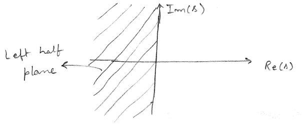
The roots of the denominator of the transfer function (\(s_1\) and \(s_2\)) are known as the poles of the transfer function and play a significant role on the dynamics of the system. For a system to be stable, the poles of the system must lie in the left half plane of the complex \(s\) plane as shown in Figure 5.1.
5.4 Nomoto’s First Order Model
Consider the transfer function for the Nomoto’s second order model shown in \(\eqref{eq-nomoto-transfer-func}\). Factorizing the denominator, the transfer function is denoted by
\[\begin{align} \frac{r_0}{\delta_0} = \frac{K(1+T_3s)}{(1 + T_1s)(1 + T_2s)} \end{align}\]
For many ships, \(T_2\) and \(T_3\) have values of similar order of magnitude. In this case, the system exhibits a first order dynamics defined by an equivalent time constant \(T\) defined as
\[\begin{align} T = T_1 + T_2 - T_3 \end{align}\]
The equivalent first order transfer function is given by
\[\begin{align} \frac{r_0}{\delta_0} = \frac{K}{1 + Ts} \label{eq-nomoto-1st-transfer-func} \end{align}\]
Expressing this transfer function in the differential form yields the Nomoto’s first order model shown in
\[\begin{align} T\dot{r} + r = K \delta \label{eq-nomoto-1st} \end{align}\]
Unlike the linearized equations of motion described in Chapter 3 that was characterized by several hydrodynamic derivatives, the Nomoto’s first order model is characterized only by two parameters \(K\) and \(T\). Physically \(K\) and \(T\) represent the rudder effectiveness and time constant respectively and can be thought of as non-dimensional ratios shown below.
\[\begin{align} T = \frac{\text{Yaw inertia}}{\text{Yaw damping}} \nonumber \end{align}\]
\[\begin{align} K = \frac{\text{Turning moment}}{\text{Yaw damping}} \nonumber \end{align}\]
For a step input of rudder angle \(\delta\) applied at \(t=0\), the solution of \(\eqref{eq-nomoto-1st}\) is shown in \(\eqref{eq-nomoto-1st-solution}\).
\[\begin{align} r(t) = K \delta (1 - e^{-\frac{1}{T}}) \label{eq-nomoto-1st-solution} \end{align}\]
As time increases, the yaw rate \(r\) increases with time at a declining exponential rate governed by \(T\) and approaches the steady state value \(K\delta\). The final turn rate does not depend on \(T\) and only depends on \(K\) and the applied step input \(\delta\).
The maneuvering characteristics can be understood intuitively through the Nomoto parameters - Nomoto time constant \(T\) and Nomoto gain \(K\). A larger \(K\) implies a greater turning ability and a smaller \(T\) implies a more responsive ship. The steady turning radius \(R\) is given by
\[\begin{align} R = \frac{U}{r} = \frac{U}{K\delta} \end{align}\]
In the non-dimensional form
\[\begin{align} R' = \frac{R}{L} = \frac{1}{r'} = \frac{1}{K'\delta} \end{align}\]
where \(K'\) is the non-dimensionalized value of \(K\) and is shown in \(\eqref{eq-Kprime}\).
\[\begin{align} K' = \frac{N_v' Y_{\delta}' - Y_v' Y_{\delta}'}{(N_r' - m'x_G') Y_v' - (Y_r' - m') N_v'} \label{eq-Kprime} \end{align}\]
The Nomoto time constant \(T\) determines the response time of the vessel. A larger \(T\) implies that the vessel takes longer time to respond to the rudder commands. This means that the ship is sluggish and harder to control.
The transfer function for the Nomoto’s first order model shown in \(\eqref{eq-nomoto-1st-transfer-func}\) has a single pole \(s_1 = -\frac{1}{T}\). If \(s_1\) lies in the left half plane, then the system response is stable. Thus the condition for straight line stability of a ship governed by Nomoto’s first order model translates to \(T>0\). Greater value of \(\frac{1}{T}\) denotes a better course stability. The Nomoto parameters \(T\) and \(K\) also provide a good basis for comparing various designs during the design spiral.
The next chapter will take a look at the turning circle maneuver, which is one of the standard maneuvers of a ship.
5.5 Exercises
A ship has a Nomoto gain \(K = -0.5\) /s and is given a rudder angle \(\delta = 10^{\circ}\). Calculate the steady-state yaw rate \(r\).
For a ship traveling at \(10\) m/s with a Nomoto gain \(K = -0.3\) /s and rudder angle \(\delta = 15^{\circ}\), calculate the steady turning radius \(R\).
A ship has a Nomoto time constant \(T = 5\) s. After a step input of rudder angle, how long will it take for the ship to reach \(63.2\%\) of its steady-state yaw rate?
Given a vessel with dynamics governed by first-order Nomoto model with \(K = -0.4\) /s and \(T = 8\) s, calculate the yaw rate \(r\) after \(4\) seconds when a step input of \(\delta = -20^{\circ}\) is applied.
A ship has parameters \(T_1 = 10\) s, \(T_2 = 3\) s, and \(T_3 = 2\) s. Calculate the equivalent time constant \(T\) for the first-order Nomoto model.
For a ship with length \(L = 100\) m, non-dimensional Nomoto gain \(K' = -2.5\), and rudder angle \(\delta = -5^{\circ}\), calculate the turning radius \(R\).
Given a ship with \(K = -0.6\) /s and \(T = 6\) s, calculate what percentage of the steady-state yaw rate will be achieved after \(12\) seconds for an applied step input of \(\delta = -10^{\circ}\).
A ship has parameters \(T_1 = 15\) s and \(T_2 = 5\) s. Determine the location of the poles of the transfer function for the second-order Nomoto model and comment on the stability of the system.
Two ships have the same Nomoto gain \(K = -0.4\) /s but different time constants \(T_A = 4\) s and \(T_B = 8\) s. Compare their responsiveness by calculating the yaw rate ratio at \(t = 1\) s for a step input of \(\delta = -5^{\circ}\). Which ship responds faster and by what factor?
For a ship with \(K = -0.5\) /s and \(T = 10\) s, calculate the phase lag \(\epsilon\) when subjected to a sinusoidal rudder input with frequency \(\omega = 0.1\) rad/s.
Consider a second-order Nomoto model with \(T_1 = 12\) s, \(T_2 = 4\) s, \(T_3 = 3\) s, and \(K = -0.3\) /s. For a sinusoidal input \(\delta(t) = 10^{\circ} \cos(0.2t)\), determine:
- The amplitude ratio \(|r_0/\delta_0|\)
- The phase lag \(\epsilon\)
- Compare these results with the equivalent first-order model
A ship has the following non-dimensional parameters: \(m' = 0.2\), \(x_G' = 0.1\), \(Y_v' = -0.4\), \(Y_r' = 0.15\), \(N_v' = -0.05\), \(N_r' = -0.1\), \(Y_\delta' = 0.3\). Calculate the turning radius \(R\) for a rudder angle \(\delta = 5^{\circ}\) if the length of the ship is \(L = 100\) m.
Consider a second order Nomoto model that has the following transfer function:
\[\begin{align} \frac{r_0}{\delta_0} = -\left(\frac{0.3 + 0.9s}{1 + 16s + 48s^2}\right) \nonumber \end{align}\]
- Locate the poles of the transfer function and comment on the stability of the system
- What is the yaw rate amplitude for a sinusoidal rudder input with amplitude \(\delta_0 = 5^{\circ}\) and frequency \(\omega = 0.1\) rad/s?
- What is the phase lag of the system for the same input?
Consider a second-order Nomoto model that has the following transfer function:
\[\begin{align} \frac{r_0}{\delta_0} = -\left(\frac{0.3 + 0.9s}{1 + 4s + 8s^2}\right) \nonumber \end{align}\]
- Locate the poles of the transfer function and comment on the stability of the system
- Determine the time constants of the system
- Write down the equivalent first-order transfer function
- Cut-off frequency for a system is defined as the frequency at which the amplitude ratio is \(\frac{1}{\sqrt{2}}\) of the steady-state value (value at \(\omega = 0\)). Determine the cut-off frequency for the first-order model. How is this related to the equivalent time constant?
- Programming Exercise: Plot the magnitude of the amplitude ratio and the phase lag for the second-order and first-order models for the frequency range \(0.01 \leq \omega \leq 10\) rad/s. Plot the curves on a log-log scale. This is also known as the Bode plot. Mark the cut-off frequency for both the models on the plot. What do you observe from the plot?
Consider a \(150\) m long vessel operating at a design speed of \(10\) m/s with the non-dimensional Nomoto parameters \(K' = -2.5\) and \(T' = 0.5\). Calculate the steady state yaw rate at time \(t = 15\) s for a sinusoidal rudder input given by \(\delta(t) = 15^{\circ} \sin(t/10)\).
Answer Key
The steady-state yaw rate is \(-0.0873\) rad/s
The steady turning radius is \(-127.32\) m
The time to reach \(63.2\%\) of the steady-state yaw rate is \(5.00\) seconds
The yaw rate after \(4\) seconds is \(0.0549\) rad/s
The equivalent time constant is \(11.00\) seconds
The turning radius is \(458.37\) m
The percentage of the steady-state yaw rate is \(86.47%\)
The poles of the transfer function are \(-0.07\) and \(-0.20\)
The ship with time constant \(4.00\) seconds is more responsive by a factor of \(0.53\)
The phase lag is \(-135.00^{\circ}\)
For the second-order model:
The amplitude ratio is \(0.60\) /s
The phase lag is \(-104.92^{\circ}\)
The amplitude ratio of the first-order model is \(0.62\) /s
The phase lag of the first-order model is \(-111.04^{\circ}\)
The turning radius is \(496.56\) m
For the second-order model:
The poles of the transfer function are \(-0.08\) and \(-0.25\). The system is stable.
The yaw rate amplitude is \(0.02\) rad/s
The phase lag is \(-124.70^{\circ}\)
For the second-order model:
The poles of the transfer function are \(-0.25+0.25j\) and \(-0.25-0.25j\). The system is stable.
The time constants of the system are \(T_1 = 2.00+2.00j\) s, \(T_2 = 2.00-2.00j\) s and \(T_3 = 3.00\) s.
The equivalent first-order transfer function is \(\frac{-0.30}{1 + 1.00s}\)
The cut-off frequency for the first-order model is \(\omega_c = 1.00\) rad/s. This is related to the equivalent time constant \(T = T_1 + T_2 - T_3\) by \(\omega_c = 1/T\).
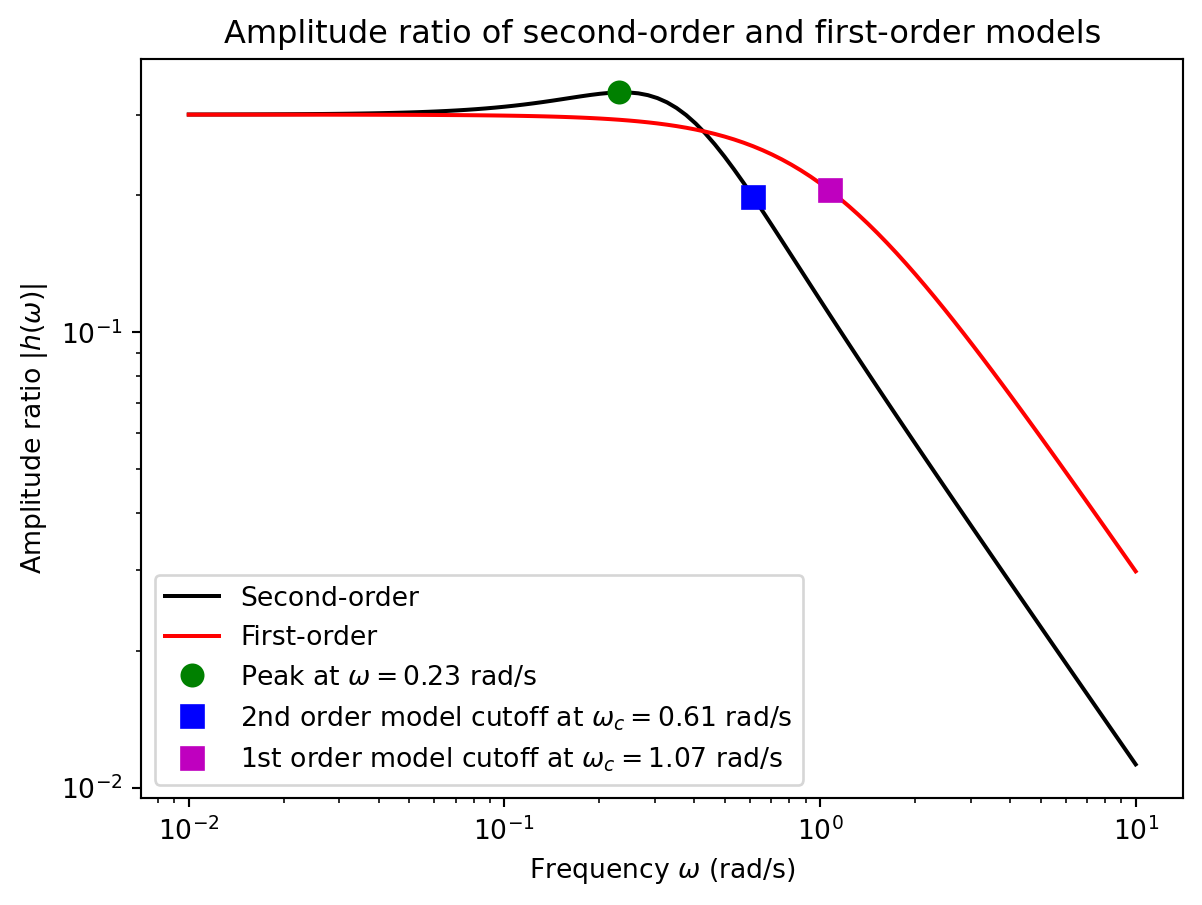
This plot of the amplitude ratio \(h(\omega) = r_0/\delta_0\) is also known as the Bode plot.
Notice that the amplitude ratio for the second-order model here exhibits a peak value greater than the steady-state value at low frequencies. This is a characteristic that can be exhibited only by a second-order system. A first order system will exhibit a monotonically decreasing amplitude ratio with increasing frequency. Also, while the the first order model behaves in a similar manner to the second order model at low frequencies, it exhibits significantly different behavior at high frequencies.
You can further notice that both the first and second order models behave like a low-pass filter. Inputs with higher frequencies are attenuated more than lower frequencies. This means that faster rudder variations will not affect the yaw response as much as slower variations. This also physically makes sense as the ship, due to its inertia, will not have sufficient time to react to faster variations. The curve for both models taper off to a straight line at high frequencies. Since the plot is on a log-log scale, this straight line means that the amplitude ratio decreases almost linearly with increasing frequency.
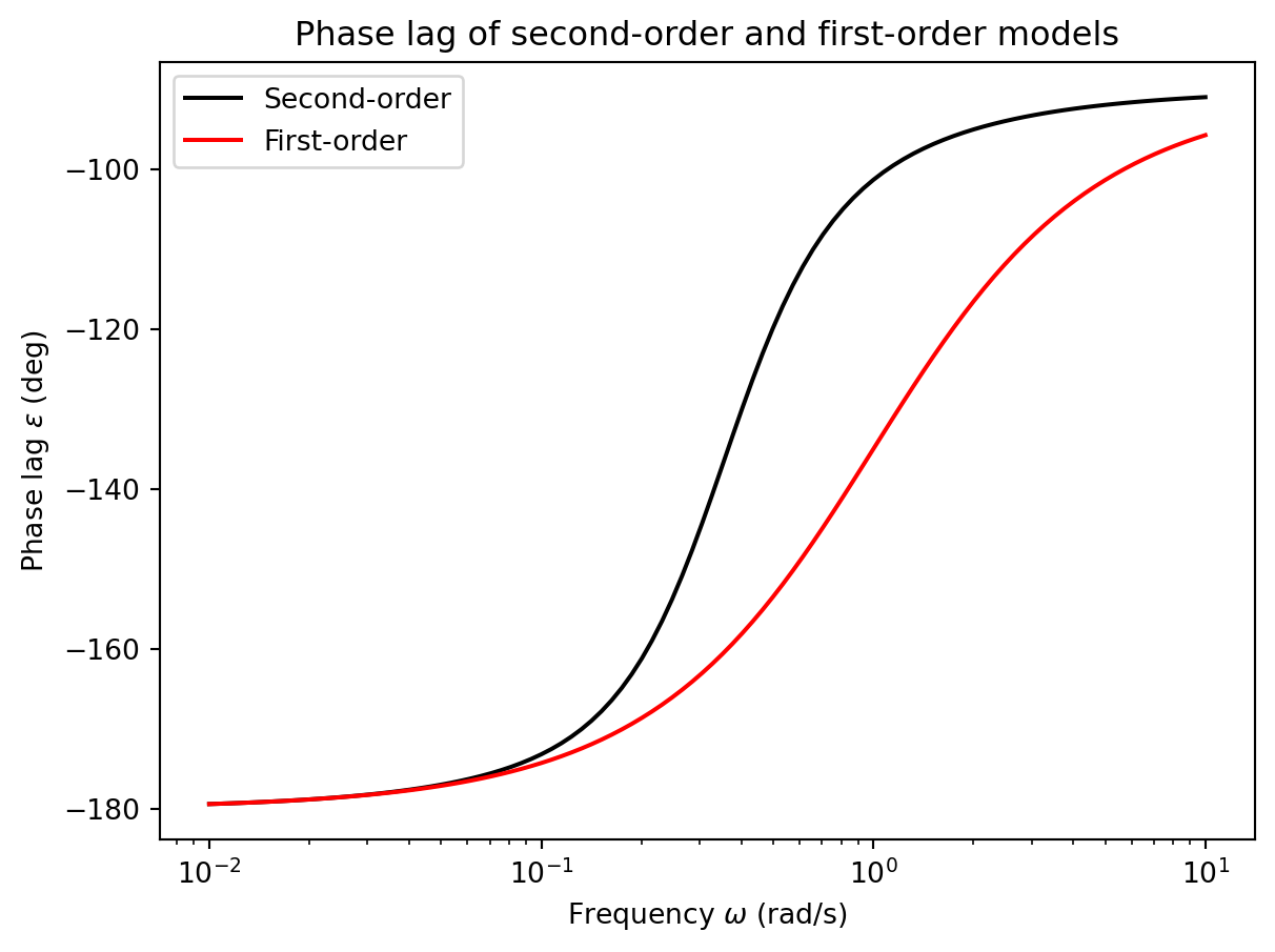
At higher frequencies, the slope of the second order model is steeper than that of the first order model. However, the phase lag of the second order model is higher than that of the first order model. This means that the response of the second order model will lag more than the first order model for higher frequency inputs.
The steady state yaw rate at \(t = 15\) s is \(-0.0435\) rad/s