2  Rigid Body Dynamics

Motion of any general rigid body is governed by conservation of linear and angular momenta (Newton’s second law of motion). The derivation of the dynamic equations of motion for a rigid body can be separated into two steps:

• The application of conservation of linear momemtum yields the translational equations of motion (also known as Newton’s equations for a rigid body). In this step the vehicle is assumed to be a point mass whose mass is assumed to be concentrated at the center of gravity \(G\).
• The application of conservation of angular momemtum yields the rotational euations of motion (also known as Euler’s equations for a rigid body). In this step the mass distribution of the rigid body plays a role in the dynamics.

The two set of equations obtained above are referred to as Newton-Euler equations of motion.

2.1 Translational Equations of Motion

Figure 2.1

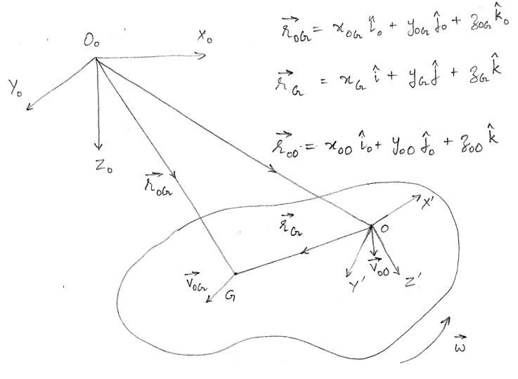
Consider a rigid body that is both translating and rotating as shown in Figure 2.1, whose center of gravity is denoted by \(G\) and the BCS origin is denoted by \(O\). The GCS frame is depicted as \(X_0Y_0Z_0\) with origin at \(O_0\) and the BCS frame is depicted as \(X'Y'Z'\) with origin \(O\). The three unit vectors along GCS are denoted as \((\hat{i}_0, \hat{j}_0, \hat{k}_0)\) and the corresponding unit vectors along BCS are denoted as \((\hat{i}, \hat{j}, \hat{k})\). The position vector from GCS origin to BCS origin expressed in GCS is denoted as shown in \(\eqref{eq-bcs-origin-vec-gcs}\). The position vector from GCS origin to center of gravity \(G\) expressed in GCS is denoted as shown in \(\eqref{eq-cog-vec-gcs}\). Let vector from BCS origin to the center of gravity \(G\) expressed in BCS be denoted as shown in \(\eqref{eq-cog-vec-bcs}\).

\[\begin{align} \vec{r}_{0O} = x_{0O} \hat{i}_0 + x_{0O} \hat{j}_0 + z_{0O} \hat{k}_0 \label{eq-bcs-origin-vec-gcs} \end{align}\]

\[\begin{align} \vec{r}_{0G} = x_{0G} \hat{i}_0 + x_{0G} \hat{j}_0 + z_{0G} \hat{k}_0 \label{eq-cog-vec-gcs} \end{align}\]

\[\begin{align} \vec{r}_G = x_G \hat{i} + y_G \hat{j} + z_G \hat{k} \label{eq-cog-vec-bcs} \end{align}\]

Let the velocity and acceleration of the center of gravity \(G\) expressed in GCS and BCS be denoted by \((\vec{v}_{0G}, \vec{a}_{0G})\) and \((\vec{v}_{G}, \vec{a}_{G})\) respectively. Similarly the angular velocity of the body expressed in GCS and BCS be denoted by \((\vec{\omega}_0, \vec{\alpha}_0)\) and \((\vec{\omega}, \vec{\alpha})\) respectively. Let the velocity and acceleration of the BCS origin \(O\) expressed in GCS and BCS be denoted by \((\vec{v}_{0O}, \vec{a}_{0O})\) and \((\vec{v}, \vec{a})\) respectively. Note that from the previous chapter, the vectors \(\vec{v}\) and \(\vec{\omega}\) are denoted as shown in \(\eqref{eq-vel-bcs}\) and \(\eqref{eq-ang-vel-bcs}\) respectively.

\[\begin{align} \vec{v} = u\hat{i} + v\hat{j} + w\hat{k} = \{v_1\} \label{eq-vel-bcs} \end{align}\]

\[\begin{align} \vec{\omega} = p\hat{i} + q\hat{j} + r\hat{k} = \{v_2\} \label{eq-ang-vel-bcs} \end{align}\]

It can be seen that the position vector \(\vec{r}_{0G}\) can be expressed as shown in \(\eqref{eq-position-vec-triangle-law}\) where \(\boldsymbol{R}\) is the rotation matrix as defined in \(\eqref{eq-rotm-expansion}\).

\[\begin{align} \vec{r}_{0G} = \vec{r}_{0O} + \boldsymbol{R} \vec{r}_G \label{eq-position-vec-triangle-law} \end{align}\]

Differentiating \(\eqref{eq-position-vec-triangle-law}\) with respect to time yields \(\eqref{eq-vel-triangle-law}\).

\[\begin{align} \vec{v}_{0G} = \vec{v}_{0O} + \dot{\boldsymbol{R}} \vec{r}_G + \boldsymbol{R} \dot{\vec{r}}_G \label{eq-vel-triangle-law} \end{align}\]

Note that \(\dot{\vec{r}}_G = 0\) as in the BCS frame, the location of center of gravity \(G\) will not vary with time due to the rigid body assumption. The vector \(\vec{r}_G\) can be expressed from \(\eqref{eq-position-vec-triangle-law}\) as shown in \(\eqref{eq-rG-recast}\).

\[\begin{align} \vec{r}_G = \boldsymbol{R}^T (\vec{r}_{0G} - \vec{r}_{0O}) \label{eq-rG-recast} \end{align}\]

Substituting into \(\eqref{eq-vel-triangle-law}\) yields \(\eqref{eq-vel-triangle-law-1}\).

\[\begin{align} \vec{v}_{0G} = \vec{v}_{0O} + \dot{\boldsymbol{R}} \boldsymbol{R}^T (\vec{r}_{0G} - \vec{r}_{0O}) \label{eq-vel-triangle-law-1} \end{align}\]

The product \(\dot{\boldsymbol{R}} \boldsymbol{R}^T\) can be evaluated using symbolic python (sympy package) as seen in the code give below and the final expression in summarized in a compact form in \(\eqref{eq-RdotRT-compact-1}\). Note that \(s_1 = \sin(\phi)\), \(c_1 = \cos(\phi)\), \(s_2 = \sin(\theta)\), \(c_2=\cos(\theta)\), \(s_3 = \sin(\psi)\) and \(c_3 = \cos(\psi)\).

import sympy as sp

# Define symbols for angles and their time derivatives
phi, theta, psi = sp.symbols('phi theta psi', cls=sp.Function)
t = sp.symbols('t')
phi = phi(t)
theta = theta(t)
psi = psi(t)

# Define derivatives of angles with respect to time
phi_dot = sp.diff(phi, t)
theta_dot = sp.diff(theta, t)
psi_dot = sp.diff(psi, t)

# Define trigonometric functions
s1, c1 = sp.sin(phi), sp.cos(phi)
s2, c2 = sp.sin(theta), sp.cos(theta)
s3, c3 = sp.sin(psi), sp.cos(psi)

# Define the rotation matrix R
R = sp.Matrix([
    [c2*c3, -c1*s3 + s1*s2*c3, s1*s3 + c1*s2*c3],
    [c2*s3, c1*c3 + s1*s2*s3, -s1*c3 + c1*s2*s3],
    [-s2, s1*c2, c1*c2]
])

# Compute the time derivative of R
R_dot = R.diff(t)

# Compute R^T
R_T = R.transpose()

# Compute R_dot * R_T
result = R_dot * R_T

# Simplify the result
simplified_result = sp.simplify(result)
simplified_result

\[\begin{align} \dot{\boldsymbol{R}} \boldsymbol{R}^T = \begin{bmatrix} 0 & s_2\dot{\phi} - \dot{\psi} & s_3c_2\dot{\phi} + c_3\dot{\theta} \\ -s_2\dot{\phi} + \dot{\psi} & 0 & s_3\dot{\theta} - c_3c_2\dot{\phi} \\ -s_3c_2\dot{\phi} - c_3\dot{\theta} & -s_3\dot{\theta} + c_3c_2\dot{\phi} & 0 \end{bmatrix} \label{eq-RdotRT-compact-1} \end{align}\]

From the previous chapter it is seen that the angular velocity of the body \(\vec{\omega}\) is related to the Euler rates by \(\eqref{eq-ang-vel-bcs-repeat}\).

\[\begin{align} \vec{\omega} = \begin{bmatrix} \dot{\phi} - s_2 \dot{\psi} \\ c_1 \dot{\theta} + s_1c_2 \dot{\psi} \\ -s_1 \dot{\theta} + c_1c_2 \dot{\psi} \end{bmatrix} \label{eq-ang-vel-bcs-repeat} \end{align}\]

The angular velocity of the body expressed in GCS will be given by \(\eqref{eq-ang-vel-gcs}\). Note that the following code has been used to evaluate the final expression shown in \(\eqref{eq-ang-vel-gcs}\).

import sympy as sp

# Define symbols for angles and their time derivatives
phi, theta, psi = sp.symbols('phi theta psi', cls=sp.Function)
t = sp.symbols('t')
phi = phi(t)
theta = theta(t)
psi = psi(t)

# Define derivatives of angles with respect to time
phi_dot = sp.diff(phi, t)
theta_dot = sp.diff(theta, t)
psi_dot = sp.diff(psi, t)

# Define trigonometric functions
s1, c1 = sp.sin(phi), sp.cos(phi)
s2, c2 = sp.sin(theta), sp.cos(theta)
s3, c3 = sp.sin(psi), sp.cos(psi)

# Define the rotation matrix R
R = sp.Matrix([
    [c2*c3, -c1*s3 + s1*s2*c3, s1*s3 + c1*s2*c3],
    [c2*s3, c1*c3 + s1*s2*s3, -s1*c3 + c1*s2*s3],
    [-s2, s1*c2, c1*c2]
])

# Define angular velocity omega in BCS
omega = sp.Matrix([[phi_dot - s2*psi_dot], 
            [c1*theta_dot + s1*c2*psi_dot], 
            [-s1*theta_dot + c1*c2*psi_dot]])

# Angular velocity in GCS omega_0
omega_0 = R * omega

# Simplify the result
simplified_result = sp.simplify(omega_0)
simplified_result

\[\begin{align} \vec{\omega}_0 = \boldsymbol{R} \vec{\omega} = \begin{bmatrix} -s_3 \dot{\theta} + c_2c_3\dot{\phi} \\ s_3c_2\dot{\phi} + c_3 \dot{\theta} \\ - s_2 \dot{\phi} + \dot{\psi} \end{bmatrix} \label{eq-ang-vel-gcs} \end{align}\]

Expressing cross product as a matrix multiplication

Consider two vectors \(\vec{a} = a_1 \hat{i} + a_2 \hat{j} + a_3 \hat{k}\) and \(\vec{b} = b_1 \hat{i} + b_2 \hat{j} + b_3 \hat{k}\). The cross product \(\vec{a} \times \vec{b}\) is given by

\[\begin{align} \vec{a} \times \vec{b} = \begin{vmatrix} \hat{i} & \hat{j} & \hat{k} \\ a_1 & a_2 & a_3 \\ b_1 & b_2 & b_3 \end{vmatrix} = (a_2b_3 - a_3b_2) \hat{i} + (a_3b_1 - a_1b_3) \hat{j} + (a_1b_2 - a_2b_1) \hat{k} \end{align}\]

A skew symmetric matrix constructed from a vector is defined as

\[\begin{align} \boldsymbol{S}(\vec{a}) = \begin{bmatrix} 0 & -a_3 & a_2 \\ a_3 & 0 & -a_1 \\ -a_2 & a_1 & 0 \end{bmatrix} \end{align}\]

It can then be seen that the cross product \(\vec{a} \times \vec{b}\) can be expressed as

\[\begin{align} \vec{a} \times \vec{b} = \begin{bmatrix} a_2b_3 - a_3b_2 \\ a_3b_1 - a_1b_3 \\ a_1b_2 - a_2b_1 \end{bmatrix} = \begin{bmatrix} 0 & -a_3 & a_2 \\ a_3 & 0 & -a_1 \\ -a_2 & a_1 & 0 \end{bmatrix} \begin{bmatrix} b_1\\ b_2\\ b_3 \end{bmatrix} = \boldsymbol{S}(\vec{a}) \vec{b} \end{align}\]

Similarly,

\[\begin{align} \vec{a} \times \vec{b} = \begin{bmatrix} a_2b_3 - a_3b_2 \\ a_3b_1 - a_1b_3 \\ a_1b_2 - a_2b_1 \end{bmatrix} = \begin{bmatrix} 0 & b_3 & -b_2 \\ -b_3 & 0 & b_1 \\ b_2 & -b_1 & 0 \end{bmatrix} \begin{bmatrix} a_1\\ a_2\\ a_3 \end{bmatrix} = -\boldsymbol{S}(\vec{b})\vec{a} \end{align}\]

It can be seen that the right hand side of \(\eqref{eq-RdotRT-compact-1}\) is a skew symmetric matrix constructed from \(\vec{\omega}_0\) shown in \(\eqref{eq-ang-vel-gcs}\). Using the property of expressing cross product as a matrix multiplication, \(\eqref{eq-vel-triangle-law-1}\) can be written as shown in \(\eqref{eq-vel-triangle-law-2}\).

\[\begin{align} \vec{v}_{0G} = \vec{v}_{0O} + \vec{\omega}_0 \times (\vec{r}_{0G} - \vec{r}_{0O}) \label{eq-vel-triangle-law-2} \end{align}\]

Differentiating \(\eqref{eq-vel-triangle-law-2}\) with respect to time again yields \(\eqref{eq-acc-triangle-law-1}\).

\[\begin{align} \vec{a}_{0G} = \vec{a}_{0O} + \vec{\alpha}_0 \times (\vec{r}_{0G} - \vec{r}_{0O}) + \vec{\omega}_0 \times (\vec{v}_{0G} - \vec{v}_{0O}) \label{eq-acc-triangle-law-1} \end{align}\]

Substituting \((\vec{v}_{0G} - \vec{v}_{0O})\) from \(\eqref{eq-vel-triangle-law-2}\) into \(\eqref{eq-acc-triangle-law-1}\) yields \(\eqref{eq-acc-triangle-law-2}\).

\[\begin{align} \vec{a}_{0G} = \vec{a}_{0O} + \vec{\alpha}_0 \times (\vec{r}_{0G} - \vec{r}_{0O}) + \vec{\omega}_0 \times (\vec{\omega}_0 \times (\vec{r}_{0G} - \vec{r}_{0O})) \label{eq-acc-triangle-law-2} \end{align}\]

Newton’s second law for a point mass can be written as \(\eqref{eq-newtons-2nd-law}\) where \(\vec{F}_{0}\) is the force acting on the body expressed in GCS. \(m\) denotes the mass of the rigid body.

\[\begin{align} m \vec{a}_{0G} = \vec{F}_{0} \label{eq-newtons-2nd-law} \end{align}\]

Sustituting the acceleration of \(G\) expressed in GCS from \(\eqref{eq-acc-triangle-law-2}\) leads to \(\eqref{eq-newtons-eom}\).

\[\begin{align} m \left[\vec{a}_{0O} + \vec{\alpha}_0 \times (\vec{r}_{0G} - \vec{r}_{0O}) + \vec{\omega}_0 \times (\vec{\omega}_0 \times (\vec{r}_{0G} - \vec{r}_{0O}))\right] = \vec{F}_{0} \label{eq-newtons-eom} \end{align}\]

Notice that all the quantities in \(\eqref{eq-newtons-eom}\) are expressed in GCS frame. Premultiplying \(\boldsymbol{R}^T\) on both sides of \(\eqref{eq-newtons-eom}\) leads to translational equations of motion expressed in BCS frame as shown in \(\eqref{eq-newtons-eom-1}\).

\[\begin{align} m \left[\vec{a} + \vec{\alpha} \times \vec{r}_{G} + \vec{\omega} \times (\vec{\omega} \times \vec{r}_{G})\right] = \vec{F} \label{eq-newtons-eom-1} \end{align}\]

Note that \(\boldsymbol{R}^T(\vec{\alpha}_0 \times (\vec{r}_{0G} - \vec{r}_{0O})) = \vec{\alpha} \times \vec{r}_{G}\) and \(\boldsymbol{R}^T(\vec{\omega}_0 \times (\vec{\omega}_0 \times (\vec{r}_{0G} - \vec{r}_{0O}))) = \vec{\omega} \times (\vec{\omega} \times \vec{r}_{G})\). Transforming vectors to BCS and taking a cross product is equivalent to taking a cross product of vectors in GCS and transforming the resultant vector to BCS. \(\vec{F} = X \hat{i} + Y \hat{j} + Z \hat{k}\) in \(\eqref{eq-newtons-eom-1}\) represents the force acting of the rigid body expressed in BCS frame.

In BCS \(\vec{a} \neq \dot{\vec{v}}\) as BCS is a non-inertial frame of reference. Differentiation of velocity will yield acceleration only in an inertial frame. Instead \(\vec{a}\) can be expressed in terms of \(\dot{\vec{v}}\) and \(\vec{v}\) as shown in \(\eqref{eq-acc-vel-der-bcs}\).

\[\begin{align} \vec{a} = \boldsymbol{R}^T\vec{a}_{0O} = \boldsymbol{R}^T \frac{d}{dt} \vec{v}_{0O} = \boldsymbol{R}^T \frac{d}{dt} \left(\boldsymbol{R} \vec{v}\right) = \boldsymbol{R}^T\dot{\boldsymbol{R}}\vec{v} + \dot{\vec{v}} = \dot{\vec{v}} + \vec{\omega} \times \vec{v} \label{eq-acc-vel-der-bcs} \end{align}\]

Substituting \(\eqref{eq-acc-vel-der-bcs}\) into \(\eqref{eq-newtons-eom-1}\) results in the translational equations of motion in the vector form and are shown in \(\eqref{eq-newtons-eom-2}\).

\[\begin{align} m \left[\dot{\vec{v}} + \vec{\omega} \times \vec{v} + \vec{\alpha} \times \vec{r}_{G} + \vec{\omega} \times (\vec{\omega} \times \vec{r}_{G})\right] = \vec{F} \label{eq-newtons-eom-2} \end{align}\]

2.2 Rotational Equations of Motion

Let the angular momentum of the vessel about the center of gravity \(G\) expressed in GCS be denoted by \(\vec{L}_{0G}\). Let the angular momentum of the vessel about the center of gravity \(G\) expressed in BCS be denoted by \(\vec{L}_G\). Let the external moment on the vessel about the center of gravity \(G\) expressed in GCS be denoted by \(\vec{M}_{0G}\). The conservation of angular momentum for the vessel is shown by \(\eqref{eq-ang-momentum-conservation}\).

\[\begin{align} \frac{d}{dt} \vec{L}_{0G} = \vec{M}_{0G} \label{eq-ang-momentum-conservation} \end{align}\]

This can be recast as shown in \(\eqref{eq-ang-momentum-conservation-1}\).

\[\begin{align} \vec{M}_{0G} &= \frac{d}{dt} (\boldsymbol{R} \vec{L}_G) = \boldsymbol{R} \dot{\vec{L}}_G + \dot{\boldsymbol{R}} \vec{L}_G \nonumber \\ &= \boldsymbol{R} \left(\dot{\vec{L}}_G + \boldsymbol{R}^T \dot{\boldsymbol{R}} \vec{L}_{G} \right) \nonumber \\ &= \boldsymbol{R} \left(\dot{\vec{L}}_G + \vec{\omega} \times \vec{L}_{G} \right) \label{eq-ang-momentum-conservation-1} \end{align}\]

Rearranging yields \(\eqref{eq-ang-momentum-conservation-2}\).

\[\begin{align} \dot{\vec{L}}_G + \vec{\omega} \times \vec{L}_{G} = \boldsymbol{R}^T \vec{M}_{0G} \label{eq-ang-momentum-conservation-2} \end{align}\]

It is well known from rigid body mechanics that the angular momentum of the body in BCS \(\vec{L}_{G}\) can be expressed as the product of inertia tensor and the angular velocity as shown in \(\eqref{eq-ang-mom-inertia}\).

\[\begin{align} \vec{L}_{G} = \boldsymbol{I}_G \vec{\omega} \label{eq-ang-mom-inertia} \end{align}\]

The inertia tensor \(\boldsymbol{I}_G\) is defined as

\[\begin{align} \boldsymbol{I}_G = \begin{bmatrix} I_x^G & -I_{xy}^G & -I_{xz}^G \\ -I_{yx}^G & I_y^G & -I_{yz}^G \\ -I_{zx}^G & -I_{zy}^G & I_z^G \end{bmatrix} \end{align}\]

\(I_x^G\), \(I_y^G\) and \(I_z^G\) are the second mass moments of inertia. \(I_{xy}^G\), \(I_{xz}^G\), \(I_{yz}^G\), \(I_{yx}^G\), \(I_{zx}^G\) and \(I_{zy}^G\) are cross mass moments of inertia. The terms in the inertia tensor \(\boldsymbol{I}_G\) are defined with respect to a coordinate system that is parallel to the BCS but with its origin at the center of gravity \(G\).

The second mass moment of inertia \(I_x^G\) is defined as shown in \(\eqref{eq-IxG}\) where \(\mu\) represents the mass density of the body and the volume integral is performed over the volume \(V\) of the rigid body. Note that \((x - x_G)\), \((y - y_G)\) and \((z - z_G)\) represent the distance between the elemental volume \(dV\) and the center of gravity of the rigid body along directions parallel to the y and z axes of the BCS respectively. \(I_y^G\) and \(I_z^G\) are also defined in a similar manner.

\[\begin{align} I_x^G = I_{yy}^G + I_{zz}^G = \iiint_V \mu \left[(y - y_G)^2 + (z - z_G)^2\right] dV \label{eq-IxG} \end{align}\]

The cross mass moment of inertia \(I_{xy}^G\) is defined as shown in \(\eqref{eq-IxyG}\). The other terms \(I_{xz}^G\), \(I_{yz}^G\), \(I_{yx}^G\), \(I_{zx}^G\) and \(I_{zy}^G\) are defined in a similar manner.

\[\begin{align} I_{xy}^G = \iiint_V \mu (x - x_G) (y - y_G) dV \label{eq-IxyG} \end{align}\]

Note that for a rigid body \(\boldsymbol{I}_G\) is time invariant. The advantage of formulating the equations of motion in BCS is that the mass properties of the body are time invariant. On the other hand, when the equations of motion are formulated in GCS, the inertia tensor would be a time varying quantity.

Substituting \(\eqref{eq-ang-mom-inertia}\) into \(\eqref{eq-ang-momentum-conservation-2}\) results in \(\eqref{eq-rotational-eqn-cog}\).

\[\begin{align} \boldsymbol{I}_G \dot{\vec{\omega}} + \vec{\omega} \times \boldsymbol{I}_G \vec{\omega} = \boldsymbol{R}^T \vec{M}_{0G} \label{eq-rotational-eqn-cog} \end{align}\]

Let \(\vec{M} = K \hat{i} + M \hat{j} + N \hat{k}\) denote the external moment acting on the vessel about BCS origin \(O\) expressed in BCS. \(\vec{M}\) and \(\vec{M}_{0G}\) are related as shown in \(\eqref{eq-ext-moment}\) where \(\vec{F}\) is the external force acting on the body expressed in BCS.

\[\begin{align} \boldsymbol{R}^T \vec{M}_{0G} = \vec{M} - \vec{r}_G \times \vec{F} \label{eq-ext-moment} \end{align}\]

Substituting \(\eqref{eq-ext-moment}\) into \(\eqref{eq-rotational-eqn-cog}\) yields \(\eqref{eq-rotational-eqn-cog-1}\).

\[\begin{align} \boldsymbol{I}_G \dot{\vec{\omega}} + \vec{\omega} \times \boldsymbol{I}_G \vec{\omega} = \vec{M} - \vec{r}_G \times \vec{F} \label{eq-rotational-eqn-cog-1} \end{align}\]

Now \(\vec{F}\) can be substituted from \(\eqref{eq-newtons-eom-2}\) to yield \(\eqref{eq-euler-eom-1}\)

\[\begin{align} \boldsymbol{I}_G \dot{\vec{\omega}} &+ \vec{\omega} \times \boldsymbol{I}_G \vec{\omega} \nonumber \\ &= \vec{M} - \vec{r}_G \times m\left[\dot{\vec{v}} + \vec{\omega} \times \vec{v} + \vec{\alpha} \times \vec{r}_{G} + \vec{\omega} \times (\vec{\omega} \times \vec{r}_{G})\right] \label{eq-euler-eom-1} \end{align}\]

Rearranging yeilds \(\eqref{eq-euler-eom-2}\).

\[\begin{align} \boldsymbol{I}_G \dot{\vec{\omega}} &+ m \vec{r}_G \times (\dot{\vec{\omega}} \times \vec{r}_{G}) + \vec{\omega} \times \boldsymbol{I}_G \vec{\omega} \nonumber \\ &+ m \vec{r}_G \times (\vec{\omega} \times (\vec{\omega} \times \vec{r}_{G})) + m \vec{r}_G \times (\dot{\vec{v}} + \vec{\omega} \times \vec{v}) = \vec{M} \label{eq-euler-eom-2} \end{align}\]

Some of the terms can be simplified. Taking the first two terms together and applying the properties of vector cross product and expressing cross products as matrix multiplications yeilds \(\eqref{eq-inertia-simplify-1}\) and \(\eqref{eq-inertia-simplify-1a}\) respectively.

\[\begin{align} \boldsymbol{I}_G \dot{\vec{\omega}} + m \vec{r}_G \times (\dot{\vec{\omega}} \times \vec{r}_{G}) = \boldsymbol{I}_G \dot{\vec{\omega}} - m \vec{r}_G \times (\vec{r}_{G} \times \dot{\vec{\omega}}) \label{eq-inertia-simplify-1} \end{align}\]

\[\begin{align} \boldsymbol{I}_G \dot{\vec{\omega}} - m \vec{r}_G \times (\vec{r}_{G} \times \dot{\vec{\omega}}) = (\boldsymbol{I}_G - m \boldsymbol{S}(\vec{r}_G) \boldsymbol{S}(\vec{r}_G)) \dot{\vec{\omega}} = \boldsymbol{I}_O \dot{\vec{\omega}} \label{eq-inertia-simplify-1a} \end{align}\]

Note that \(\boldsymbol{I}_O\) in the last step is the inertia tensor defined with respect to BCS and is related to \(\boldsymbol{I}_G\) through the parallel axes theorem shown in \(\eqref{eq-parallel-axes-theorem}\).

\[\begin{align} \boldsymbol{I}_O = \boldsymbol{I}_G - m \boldsymbol{S}(\vec{r}_G) \boldsymbol{S}(\vec{r}_G) \label{eq-parallel-axes-theorem} \end{align}\]

Similarly, the third and fourth terms of \(\eqref{eq-euler-eom-2}\) can also be simplified using the Jacobi identity for triple cross products as shown in \(\eqref{eq-inertia-simplify-2}\), \(\eqref{eq-inertia-simplify-3}\) and \(\eqref{eq-inertia-simplify-4}\).

\[\begin{align} \vec{\omega} \times \boldsymbol{I}_G \vec{\omega} + m \vec{r}_G \times (\vec{\omega} \times (\vec{\omega} \times \vec{r}_{G})) = \vec{\omega} \times \boldsymbol{I}_G \vec{\omega} + m \vec{\omega} \times (\vec{r}_G \times (\vec{\omega} \times \vec{r}_{G})) \label{eq-inertia-simplify-2} \end{align}\]

\[\begin{align} \vec{\omega} \times \boldsymbol{I}_G \vec{\omega} + m \vec{\omega} \times (\vec{r}_G \times (\vec{\omega} \times \vec{r}_{G})) = \vec{\omega} \times \boldsymbol{I}_G \vec{\omega} - m \vec{\omega} \times (\vec{r}_G \times (\vec{r}_{G} \times \vec{\omega})) \label{eq-inertia-simplify-3} \end{align}\]

\[\begin{align} \vec{\omega} \times \boldsymbol{I}_G \vec{\omega} - m \vec{\omega} \times (\vec{r}_G \times (\vec{r}_{G} \times \vec{\omega})) = \vec{\omega} \times (\boldsymbol{I}_G - m \boldsymbol{S}(\vec{r}_G) \boldsymbol{S}(\vec{r}_G)) \vec{\omega} = \vec{\omega} \times \boldsymbol{I}_O \vec{\omega} \label{eq-inertia-simplify-4} \end{align}\]

Substituting final expressions from \(\eqref{eq-inertia-simplify-1a}\) and \(\eqref{eq-inertia-simplify-4}\) into \(\eqref{eq-euler-eom-2}\) yeilds the rotational equations in the vector form as shown in \(\eqref{eq-euler-eom-3}\).

\[\begin{align} \boldsymbol{I}_O \dot{\vec{\omega}} + \vec{\omega} \times \boldsymbol{I}_O \vec{\omega} + m \vec{r}_G \times (\dot{\vec{v}} + \vec{\omega} \times \vec{v}) = \vec{M} \label{eq-euler-eom-3} \end{align}\]

2.3 Complete Equations of Motion for a Rigid Body

The equations of motion governing the dynamics of a rigid body are given by \(\eqref{eq-newtons-eom-final}\) and \(\eqref{eq-euler-eom-final}\).

\[\begin{align} m \left[\dot{\vec{v}} + \vec{\omega} \times \vec{v} + \vec{\alpha} \times \vec{r}_{G} + \vec{\omega} \times (\vec{\omega} \times \vec{r}_{G})\right] = \vec{F} \label{eq-newtons-eom-final} \end{align}\]

\[\begin{align} \boldsymbol{I}_O \dot{\vec{\omega}} + \vec{\omega} \times \boldsymbol{I}_O \vec{\omega} + m \vec{r}_G \times (\dot{\vec{v}} + \vec{\omega} \times \vec{v}) = \vec{M} \label{eq-euler-eom-final} \end{align}\]

When expanded, these form six equations, with one corresponding to each degree of freedom and are shown in (\(\ref{eq-eom-expanded-1}\) - \(\ref{eq-eom-expanded-6}\)).

\[\begin{align} m\left[\dot{u} - vr + wq - x_G(q^2 + r^2) + y_G(pq - \dot{r}) + z_G (pr + \dot{q})\right] = X \label{eq-eom-expanded-1} \end{align}\]

\[\begin{align} m \left[\dot{v} - wp + ur - y_G (r^2 + p^2) + z_G (qr - \dot{p}) + x_G (qp + \dot{r})\right] = Y \label{eq-eom-expanded-2} \end{align}\]

\[\begin{align} m \left[\dot{w} - uq + vp - z_G(p^2 + q^2) + x_G (rp - \dot{q}) + y_G (rq + \dot{p})\right] = Z \label{eq-eom-expanded-3} \end{align}\]

\[\begin{align} I_x \dot{p} + (I_z - I_y) qr &- (\dot{r} + pq) I_{xz} + (r^2 - q^2) I_{yz} + (pr - \dot{q}) I_{xy} \nonumber \\ &+ m \left[y_G(\dot{w} - uq + vp) - z_G(\dot{v} -wp + ur)\right] = K \label{eq-eom-expanded-4} \end{align}\]

\[\begin{align} I_y \dot{q} + (I_x - I_z) rp &- (\dot{p} + qr) I_{yx} + (p^2 - r^2) I_{zx} + (qp - \dot{r}) I_{yz} \nonumber \\ &+ m \left[z_G (\dot{u} - vr + wq) - x_G (\dot{w} - uq + vp)\right] = M \label{eq-eom-expanded-5} \end{align}\]

\[\begin{align} I_z \dot{r} + (I_y - I_x) pq &- (\dot{q} + rp) I_{zy} + (q^2 - p^2) I_{xy} + (rq - \dot{p})I_{zx} \nonumber \\ &+ m \left[x_G(\dot{v} - wp + ur) - y_G(\dot{u} - vr + wq)\right] = N \label{eq-eom-expanded-6} \end{align}\]

These equations can be represented in a compact matrix form as shown in \(\eqref{eq-eom-matrix-form}\), where \(\boldsymbol{M}_{RB}\) is a \(6 \times 6\) rigid body mass matrix, \(\boldsymbol{C}_{RB}\left(\{v\}\right)\) is the \(6 \times 6\) velocity dependent Coriolis matrix and \(\{\tau_{RB}\}\) is the \(6 \times 1\) external force and moment vector.

\[\begin{align} \boldsymbol{M}_{RB} \{\dot{v}\} + \boldsymbol{C}_{RB}\left(\{v\}\right)\{v\} = \{\tau_{RB}\} \label{eq-eom-matrix-form} \end{align}\]

The rigid body mass matrix \(\boldsymbol{M}_{RB}\) is shown in \(\eqref{eq-mass-matrix}\), where \(\boldsymbol{I}_{3 \times 3}\) is a \(3 \times 3\) identity matrix.

\[\begin{align} \boldsymbol{M}_{RB} &= \begin{bmatrix} m\boldsymbol{I}_{3 \times 3} & -m \boldsymbol{S}(\vec{r}_G) \\ m \boldsymbol{S}(\vec{r}_G) & \boldsymbol{I}_O \end{bmatrix} \nonumber \\ &= \begin{bmatrix} m & 0 & 0 & 0 & mz_G & -my_G \\ 0 & m & 0 & -mz_G & 0 & mx_G\\ 0 & 0 & m & my_G & -mx_G & 0 \\ 0 & -mz_G & my_G & I_x^O & -I_{xy}^O & -I_{xz}^O \\ mz_G & 0 & -mx_G & -I_{yx}^O & I_y^O & -I_{yz}^O \\ -my_G & mx_G & 0 & -I_{zx}^O & -I_{zy}^O & I_z^O \end{bmatrix} \label{eq-mass-matrix} \end{align}\]

The Coriolis matrix can be parameterized in terms of the mass matrix as shown in \(\eqref{eq-coriolis-mass-param}\), where \(\boldsymbol{0}_{3 \times 3}\) is a \(3 \times 3\) matrix of zeros. Note that \(\boldsymbol{M}_{11} = m\boldsymbol{I}_{3 \times 3}\), \(\boldsymbol{M}_{12} = -\boldsymbol{M}_{21} = -m \boldsymbol{S}(\vec{r}_G)\) and \(\boldsymbol{M}_{22} = \boldsymbol{I}_O\).

\[\begin{align} \boldsymbol{C}_{RB} \left(\{v\}\right) = \begin{bmatrix} \boldsymbol{0}_{3 \times 3} & -\boldsymbol{S}\left(\boldsymbol{M}_{11}\vec{v}_1 + \boldsymbol{M}_{12}\vec{v}_2\right) \\ -\boldsymbol{S}\left(\boldsymbol{M}_{11}\vec{v}_1 + \boldsymbol{M}_{12}\vec{v}_2\right) & -\boldsymbol{S}\left(\boldsymbol{M}_{21}\vec{v}_1 + \boldsymbol{M}_{22}\vec{v}_2\right) \end{bmatrix} \label{eq-coriolis-mass-param} \end{align}\]

Defining a state vector of size \(12 \times 1\) as shown in \(\eqref{eq-state}\), the kinematic and dynamic equations can be expressed together as shown in \(\eqref{eq-kinematics-dynamics}\).

\[\begin{align} \{x\} = \begin{bmatrix} u & v & w & p & q & r & x_{0O} & y_{0O} & z_{0O} & \phi & \theta & \psi \end{bmatrix}^T \label{eq-state} \end{align}\]

\[\begin{align} \{\dot{x}\} = \begin{bmatrix} \{v\} \\ \{\eta\} \end{bmatrix} = \begin{bmatrix} \boldsymbol{M}_{RB}^{-1} \left(\{\tau_{RB}\} - \boldsymbol{C}_{RB}\left(\{v\}\right)\{v\}\right) \\ \boldsymbol{J}(\{\eta_2\}) \{v\} \end{bmatrix} \label{eq-kinematics-dynamics} \end{align}\]

If the external forces and moments \(\{\tau_{RB}\}\) are known, then the velocities and pose of the body can be calculated by solving the matrix differential equation shown in \(\eqref{eq-kinematics-dynamics}\).

2.4 Exercises

1. For a rigid body with mass \(m = 100\) kg and center of gravity located at \(\vec{r}_G = [0.1, -0.15, 0.2]^T\) m in BCS, calculate both the upper right and lower left \(3 \times 3\) blocks of the rigid body mass matrix \(\boldsymbol{M}_{RB}\). Verify that they are negative transposes of each other.

2. Given a rigid body with principal moments of inertia \(I_x^G = 20\) kg⋅m², \(I_y^G = 25\) kg⋅m², \(I_z^G = 30\) kg⋅m² about its center of gravity, and products of inertia \(I_{xy}^G = 2\), \(I_{xz}^G = -3\), \(I_{yz}^G = 1\) kg⋅m², construct the complete inertia tensor \(\boldsymbol{I}_G\). Is the resulting matrix symmetric?

3. A rigid body has angular velocity \(\vec{\omega} = [0.1, 0.2, 0.3]^T\) rad/s. Calculate the skew-symmetric matrix \(\boldsymbol{S}(\vec{\omega})\) and verify the properties:

   1. \(\boldsymbol{S}(\vec{\omega})^T = -\boldsymbol{S}(\vec{\omega})\),

   2. \(\boldsymbol{S}(\vec{\omega})\vec{\omega} = \vec{0}\),

   3. \(\boldsymbol{S}(\vec{\omega})\boldsymbol{S}(\vec{\omega}) = \vec{\omega}\vec{\omega}^T - \|\vec{\omega}\|^2\boldsymbol{I}_{3\times3}\).

4. For a rigid body with mass \(m = 500\) kg and center of gravity at \(\vec{r}_G = [0.3, 0.5, -0.2]^T\) m in BCS, use the parallel axis theorem to:

   1. Calculate \(\boldsymbol{S}(\vec{r}_G)\boldsymbol{S}(\vec{r}_G)\),

   2. Determine the additional inertia terms needed to transform \(\boldsymbol{I}_G\) to \(\boldsymbol{I}_O\),

   3. Show that the resulting matrix is symmetric.

5. A rigid body has linear velocity \(\vec{v} = [1, 2, -1]^T\) m/s and angular velocity \(\vec{\omega} = [0.1, 0.2, -0.15]^T\) rad/s. Calculate:

   1. The acceleration term \(\vec{\omega} \times \vec{v}\) using cross product,

   2. The same term using the skew-symmetric matrix \(\boldsymbol{S}(\vec{\omega})\),

   3. Verify both methods give the same result.

6. A rigid body has mass \(m = 200\) kg and center of gravity at \(\vec{r}_G = [0.2, -0.1, 0.15]^T\) m in BCS. If it experiences forces \(\vec{F}_1 = [100, -50, 25]^T\) N at point \(\vec{r}_1 = [0, 0, 0]^T\) m and \(\vec{F}_2 = [-30, 40, -20]^T\) N at point \(\vec{r}_2 = [0.1, 0.1, 0.1]^T\) m (both in BCS), calculate:

   1. The total force,

   2. The moment about O,

   3. The moment about G.

7. For a rigid body with angular velocity \(\vec{\omega} = [0.5, -0.3, 0.2]^T\) rad/s and inertia tensor \(\boldsymbol{I}_G\) with principal moments \([20, 25, 30]\) kg⋅m² and products of inertia \(I_{xy}^G = I_{yz}^G = I_{xz}^G = 5\) kg⋅m², calculate:

   1. \(\boldsymbol{I}_G\vec{\omega}\),

   2. \(\vec{\omega} \times \boldsymbol{I}_G\vec{\omega}\),

   3. The rotational kinetic energy \(\frac{1}{2}\vec{\omega}^T\boldsymbol{I}_G\vec{\omega}\).

8. Given a rigid body with mass \(m = 300\) kg, \(\vec{r}_G = [0.25, -0.15, 0.1]^T\) m, and \(\boldsymbol{I}_G = \text{diag}(40, 45, 50)\) kg⋅m², calculate:

   1. The complete \(6 \times 6\) rigid body mass matrix \(\boldsymbol{M}_{RB}\),

   2. Show that it is symmetric,

   3. Calculate its determinant.

9. A rigid body has linear velocity \(\vec{v} = [2, 1, -1]^T\) m/s, angular velocity \(\vec{\omega} = [0.1, -0.2, 0.15]^T\) rad/s, and center of gravity at \(\vec{r}_G = [1, -0.5, 0.3]^T\) m. Calculate:

   1. The velocity of G in BCS,

   2. The acceleration terms \(\vec{\omega} \times \vec{v}\) and \(\vec{\omega} \times (\vec{\omega} \times \vec{r}_G)\),

   3. The total acceleration of G if \(\dot{\vec{v}} = [0.1, 0.2, -0.1]^T\) m/s² and \(\dot{\vec{\omega}} = [0, 0.1, 0]^T\) rad/s².

10. For a rigid body with \(\vec{\omega} = [0.2, -0.1, 0.3]^T\) rad/s and \(\vec{r}_G = [0.5, -0.2, 0.1]^T\) m, calculate:

    1. The centripetal acceleration term \(\vec{\omega} \times (\vec{\omega} \times \vec{r}_G)\) using cross products,

    2. The same term using skew-symmetric matrices,

    3. Show that both methods yield identical results.

11. A rigid body has mass \(m = 400\) kg, center of gravity at \(\vec{r}_G = [0.3, -0.1, 0.2]^T\) m, and inertia tensor \(\boldsymbol{I}_G\) with principal moments \([50, 60, 45]\) kg⋅m² and products of inertia \(I_{xy}^G = I_{yz}^G = I_{xz}^G = 8\) kg⋅m². If it experiences force \(\vec{F} = [200, -100, 50]^T\) N and moment \(\vec{M} = [20, -10, 5]^T\) N⋅m at O, with initial velocities \(\vec{v} = [1, -0.5, 0.2]^T\) m/s and \(\vec{\omega} = [0.1, 0, -0.1]^T\) rad/s, calculate:

    1. The complete mass matrix \(\boldsymbol{M}_{RB}\),

    2. All acceleration-dependent terms,

    3. Solve for \(\dot{\vec{v}}\) and \(\dot{\vec{\omega}}\).

12. For a rigid body of mass \(m = 100\) kg, center of gravity at \(\vec{r}_G = [0.1, -0.1, 0.2]^T\) m, and inertia tensor \[\begin{align*} \boldsymbol{I}_G = \begin{bmatrix} 30 & 4 & -2 \\ 4 & 35 & 3 \\ -2 & 3 & 40 \end{bmatrix} \text{ kg⋅m²} \end{align*}\] angular velocity \(\vec{\omega} = [0.1, 0.2, 0.3]^T\) rad/s, and linear velocity \(\vec{v} = [1, -0.5, 0.2]^T\) m/s:

    1. Derive the complete expression for \(\boldsymbol{C}_{RB}(\{v\})\{v\}\),

    2. Show that \(\{v\}^T\boldsymbol{C}_{RB}(\{v\})\{v\} = 0\),

    3. Explain the physical significance of this property.

13. Given a rigid body with mass \(m = 600\) kg, \(\vec{r}_G = [0.2, 0.1, -0.1]^T\) m, and inertia tensor \[\begin{align*} \boldsymbol{I}_G = \begin{bmatrix} 500 & -25 & -30 \\ -25 & 600 & 35 \\ -30 & 35 & 650 \end{bmatrix} \text{ kg⋅m²} \end{align*}\]

    1. Derive the complete expression for the Coriolis matrix \(\boldsymbol{C}_{RB}(\{v\})\),

    2. Show that \(\dot{\boldsymbol{M}}_{RB} - 2\boldsymbol{C}_{RB}(\{v\})\) is skew-symmetric,

    3. Explain why this property is important for energy conservation.

       Hint: What should be the rate of change of kinetic energy (\(\dot{T}\)) for a rigid body that is not subject to any external forces (i.e. \(\{\tau_{RB}\}=0\))? Remember that the total kinetic energy of a rigid body is given by \(T = \frac{1}{2} \vec{v}^T \boldsymbol{M}_{RB} \vec{v}\)

14. A marine vehicle has the following inertia tensors measured about its center of gravity (G) and about the origin of BCS (O): \[\begin{align*} \boldsymbol{I}_G = \begin{bmatrix} 400 & -20 & -15 \\ -20 & 450 & 25 \\ -15 & 25 & 500 \end{bmatrix} \text{ kg⋅m²}, \quad \boldsymbol{I}_O = \begin{bmatrix} 410 & -10 & -25 \\ -10 & 475 & 30 \\ -25 & 30 & 525 \end{bmatrix} \text{ kg⋅m²} \end{align*}\] If the mass of the vehicle is \(m = 500\) kg:

    1. Determine the coordinates of the center of gravity \(\vec{r}_G = [x_G, y_G, z_G]^T\)

    2. Calculate \(\boldsymbol{S}(\vec{r}_G)\boldsymbol{S}(\vec{r}_G)\) and verify it matches with \(\frac{1}{m}(\boldsymbol{I}_O - \boldsymbol{I}_G)\)

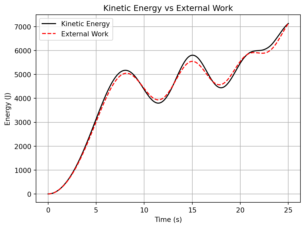
15. Programming Exercise: A marine vehicle with mass \(m = 1000\) kg, center of gravity at \(\vec{r}_G = [0.2, 0, 0.1]^T\) m, and inertia tensor \[\begin{align*} \boldsymbol{I}_G = \begin{bmatrix} 800 & 0 & -50 \\ 0 & 1200 & 0 \\ -50 & 0 & 1000 \end{bmatrix} \text{ kg⋅m²} \end{align*}\] starts from rest with initial orientation \(\phi = 20^{\circ}\), \(\theta = 30^{\circ}\), \(\psi = 45^{\circ}\) and experiences time-varying forces and moments for \(25\) seconds:

    • \(\vec{F}(t) = [500\cos\left(\frac{\pi t}{50}\right), 200\sin\left(\frac{\pi t}{50}\right), -100]^T\) N
    • \(\vec{M}(t) = [50\cos\left(\frac{\pi t}{50}\right), 30\sin\left(\frac{\pi t}{50}\right), 20]^T\) N⋅m
    1. Derive the complete equations of motion including all Coriolis terms
    2. Using RK45 integration, determine the final pose and velocities (use may explore different solvers in scipy.integrate.solve_ivp)
    3. Plot the time history of kinetic energy and verify its rate of change equals the work done by the external forces and moments.

Answer Key

1. \(\boldsymbol{M}_{12} = \begin{bmatrix} -0.00 & 20.00 & 15.00 \\ -20.00 & -0.00 & 10.00 \\ -15.00 & -10.00 & -0.00 \end{bmatrix}\) kg⋅m

   \(\boldsymbol{M}_{21} = \begin{bmatrix} 0.00 & -20.00 & -15.00 \\ 20.00 & 0.00 & -10.00 \\ 15.00 & 10.00 & 0.00 \end{bmatrix}\) kg⋅m \(= -\boldsymbol{M}_{12}^T\)

2. \(\boldsymbol{I}_{G} = \begin{bmatrix} 20.00 & -2.00 & 3.00 \\ -2.00 & 25.00 & -1.00 \\ 3.00 & -1.00 & 30.00 \end{bmatrix}\) kg⋅m²

3. 1. \(\boldsymbol{S}(\vec{\omega}) = \begin{bmatrix} 0.00 & -0.30 & 0.20 \\ 0.30 & 0.00 & -0.10 \\ -0.20 & 0.10 & 0.00 \end{bmatrix}\)

4. 1. \(\boldsymbol{S}(\vec{r}_G) \boldsymbol{S}(\vec{r}_G) = \begin{bmatrix} -0.29 & 0.15 & -0.06 \\ 0.15 & -0.13 & -0.10 \\ -0.06 & -0.10 & -0.34 \end{bmatrix}\) kg⋅m²

   2. \(\boldsymbol{I}_{O} - \boldsymbol{I}_{G} = \begin{bmatrix} 145.00 & -75.00 & 30.00 \\ -75.00 & 65.00 & 50.00 \\ 30.00 & 50.00 & 170.00 \end{bmatrix}\) kg⋅m²

5. \(\vec{\omega} \times \vec{v} = \begin{bmatrix} 0.10 \\ -0.05 \\ 0.00 \end{bmatrix}\) m/s²

6. 1. \(\boldsymbol{F}_{total} = \begin{bmatrix} 70.00 \\ -10.00 \\ 5.00 \end{bmatrix}\) N

   2. \(\boldsymbol{M}_{O} = \begin{bmatrix} -6.00 \\ -1.00 \\ 7.00 \end{bmatrix}\) N⋅m

   3. \(\boldsymbol{M}_{G} = \begin{bmatrix} -7.00 \\ -10.50 \\ 2.00 \end{bmatrix}\) N⋅m

7. 1. \(\boldsymbol{I}_G \vec{\omega} = \begin{bmatrix} 10.50 \\ -11.00 \\ 5.00 \end{bmatrix}\) kg⋅m²/s

   2. \(\vec{\omega} \times (\boldsymbol{I}_G \times \vec{\omega}) = \begin{bmatrix} 0.70 \\ -0.40 \\ -2.35 \end{bmatrix}\) kg⋅m²/s²

   3. \(T_R = 4.775\) J

8. 1. Mass matrix \(\boldsymbol{M}_{RB} = \begin{bmatrix} 300.00 & 0.00 & 0.00 & -0.00 & 30.00 & 45.00 \\ 0.00 & 300.00 & 0.00 & -30.00 & -0.00 & 75.00 \\ 0.00 & 0.00 & 300.00 & -45.00 & -75.00 & -0.00 \\ 0.00 & -30.00 & -45.00 & 49.75 & 11.25 & -7.50 \\ 30.00 & 0.00 & -75.00 & 11.25 & 66.75 & 4.50 \\ 45.00 & 75.00 & 0.00 & -7.50 & 4.50 & 75.50 \end{bmatrix}\)

   2. Is symmetric: True

   3. Determinant: \(243 \times 10^{10}\)

9. 1. Velocity of G \(\{v_G\} = \begin{bmatrix} 2.02 \\ 1.12 \\ -0.85 \end{bmatrix}\) m/s

   2. Acceleration terms: \(\boldsymbol{\omega} \times \boldsymbol{v} = \begin{bmatrix} 0.05 \\ 0.40 \\ 0.50 \end{bmatrix}\) m/s²

      \(\boldsymbol{\omega} \times (\boldsymbol{\omega} \times \boldsymbol{r}_G) = \begin{bmatrix} -0.05 \\ -0.01 \\ 0.01 \end{bmatrix}\) m/s²

   3. Total acceleration of G \(\{a_G\} = \begin{bmatrix} 0.13 \\ 0.59 \\ 0.32 \end{bmatrix}\) m/s²

10. Centripetal acceleration vector is given by:

    \(\boldsymbol{\omega} \times (\boldsymbol{\omega} \times \boldsymbol{r}_G) = \begin{bmatrix} -0.04 \\ 0.01 \\ 0.03 \end{bmatrix}\) m/s²

11. \(\dot{v} = \begin{bmatrix} 0.64 \\ -0.20 \\ 0.02 \end{bmatrix}\) m/s² and \(\dot{\omega} = \begin{bmatrix} 0.05 \\ -0.54 \\ 0.25 \end{bmatrix}\) rad/s²

12. 1. \(\boldsymbol{C}_{RB}\{v\} = \begin{bmatrix} 18.10 \\ 30.40 \\ -26.30 \\ -3.46 \\ 5.97 \\ 5.04 \end{bmatrix}\)

    2. \(\{v\}^T \boldsymbol{C}_{RB}\{v\} = 0.00\)

    3. This property shows that the Coriolis forces and moments \(\boldsymbol{C}_{RB}\{v\}\) does no work preserving energy in the absence of external forces

13. 1. \(\dot{\boldsymbol{M}}_{RB} - 2\boldsymbol{C}_{RB} = \begin{bmatrix} -0.0 & -0.0 & -0.0 & 0.0 & -2364.0 & -3516.0 \\ -0.0 & -0.0 & -0.0 & 2364.0 & 0.0 & -4740.0 \\ -0.0 & -0.0 & -0.0 & 3516.0 & 4740.0 & 0.0 \\ 0.0 & -2364.0 & -3516.0 & 0.0 & 779.2 & -690.8 \\ 2364.0 & 0.0 & -4740.0 & -779.2 & 0.0 & 43.2 \\ 3516.0 & 4740.0 & 0.0 & 690.8 & -43.2 & 0.0 \end{bmatrix}\)

    2. Is Property verified: True

    3. The skew-symmetry of \(\dot{\boldsymbol{M}}_{RB} - 2\boldsymbol{C}_{RB}\) ensures that the rate of change of kinetic energy is zero when there are no external forces or moments.

14. Two possible solutions exist and both are valid.

    Solution 1: \(r_G = \begin{bmatrix} 0.20 \\ -0.10 \\ 0.10 \end{bmatrix}\)

    Solution 2: \(r_G = \begin{bmatrix} -0.20 \\ 0.10 \\ -0.10 \end{bmatrix}\)

15.