4 Controls Fixed Stability
Consider a vessel operating in the nominal operating condition of moving steadily forward with design speed \(U\). Maneuvering stability is defined in terms of subjecting the nominal operating condition to a impulsive disturbance and observing the motion characteristics post the application of disturbance. Different types of stability are defined in terms of the characteristics of the initial state of equilibrium retained in the path after the introduction of the disturbance.
This chapter will focus on stability of the linear maneuvering dynamics derived in the previous chapter. Stability will be discussed qualitatively as well as quantitatively. The characteristics determining maneuvering stability will also be discussed.
4.1 Straight Line of Dynamic Stability
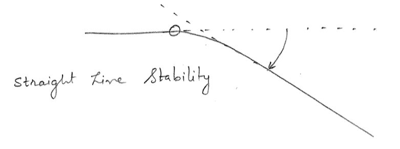
A vessel is said to have straight line or dynamic stability if the final path after release from a disturbance is a straight line but not necessarily in the same direction as the initial path. The path of a straight line stable ship before and after disturbance is shown in Figure 4.1.
4.2 Directional Stability
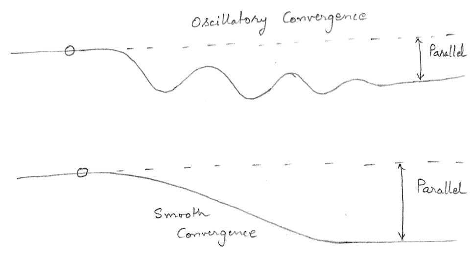
A vessel is said to have directional stability if the final path after release from a disturbance is a straight line parallel to the initial path. Note that the final path is not necessarily the same as the initial path. The path of a directional stable ship is shown in Figure 4.2.
4.3 Positional Stability
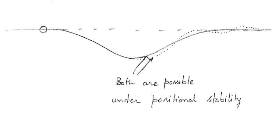
A vessel is said to be positionally stable if the final path after release from a disturbance if the same straight line that it was following prior to the introduction of disturbance. The path of a positionally stable ship is shown in Figure 4.3. Note that two possible paths are shown in Figure 4.3. The first path indicated as a solid line smoothly comes back to the original path (shown as a dashed line) without any oscillations. The second path indicated as a dotted line also comes back to the original path (shown as a dashed line) but has a decaying oscillatory behavior. Under both conditions, the vessel is said to possess positional stability.
Note that a directionally stable vessel is also straight line stable. Similarly, a positionally stable ship is both directionally stable and straight line stable.
4.4 Controls Fixed and Controls Working Stability
When discussing stability it is also important to know if the stability is being discussed in the context of:
- Controls fixed stability
- Controls working stability
Controls fixed stability means the stability of a vessel is being evaluated while all control surfaces of the vehicle are not in operation. On the other hand, controls working stability refers to the application of control systems in the evaluation of stability of the system. In terms of a ship moving in horizontal plane, the control surface is the rudder. The stability characteristics of a ship when the rudder is fixed at \(\delta = 0\) will determine its controls fixed stability. When the rudder is operational and can be utilized to counteract the disturbance effects, the stability of the system will be controls working stability.
4.5 Examples of Different Stabilities
Some examples are listed below to provide a more intuitive understanding of straight line, directional and positional stability in the context of controls fixed and controls working stability.
A surface vessel floating on the water surface possesses positional stability in vertical modes of motion. Without any actuation from a control surface, the vehicle come back to its equilibrium when disturbed in the vertical modes of motion (heave, roll and pitch) due to hydrostatic restoring forces and moments.
A hydrofoil boat has no controls fixed positional stability in the vertical modes when the weight of the boat is supported completely by the hydrofoils. With a well designed control system, the hydrofoil boat can achieve positional stability.
A neutrally buoyant submarine with non-coincident VCG (vertical center of gravity) and VCB (vertical center of buoyancy) is directionally stable in the vertical plane with its controls fixed. If we disturb the submarine from a certain depth to a different depth, it will stay at that depth, but due to non-coincident VCG and VCB it will adjust to remain horizontal. With control action such as ballast tank filling, positional stability can be achieved.
A self propelled ship does not possess positional or directional stability in the horizontal modes of motion (surge, sway and heave) with controls fixed. To achieve either, control actions like application of rudder are required.
A sailing ship driven purely by the wind possesses directional stability. When disturbed from being in the direction of the wind, the forces on the sail will orient the vessel back in the direction of the wind.
A ship towed by a tugboat possesses controls fixed positional stability. Due to the tow line, the vessel will return to follow the towline direction when disturbed. However, there is the interesting instability phenomenon of fishtailing that results in periodic or even chaotic oscillations when the conditions are right. In such cases, positional stability is lost. Some interesting papers that describe fishtailing are -
For a self propelled ship with controls fixed, only straight line stability is possible in the horizontal modes of motion. Directional and positional stability will require control actuation. This chapter will focus on ascertaining what parameters affect straight line stability of a ship and how to quantify the stability using the linearized equations of motion described in the previous chapter.
As the focus of this chapter is on straight line stability in the context of maneuvering motions, controls fixed stability will henceforth refer to controls fixed straight line stability unless explicitly stated otherwise.
4.6 Quantification of Straight Line Stability
For a controls fixed case \(\delta=0\) the linearized steering equations are given by \(\eqref{eq-sway-controls-fixed}\) and \(\eqref{eq-yaw-controls-fixed}\).
\[\begin{align} (m - Y_{\dot{v}}) \dot{v} - (Y_{\dot{r}} - m x_G) \dot{r} - Y_v v - (Y_r - mU) r = 0 \label{eq-sway-controls-fixed} \end{align}\]
\[\begin{align} (I_z - N_{\dot{r}}) \dot{r} - (N_{\dot{v}} - m x_G) \dot{v} - N_v v - (N_r - mx_GU) r = 0 \label{eq-yaw-controls-fixed} \end{align}\]
Since the above system of equations are linear, linear superposition of solutions is valid and hence an exponential solution can be assumed as shown below
\[\begin{align} v = v_0 e^{st} \quad \dot{v} = sv_0 e^{st} \nonumber \\ r = r_0 e^{st} \quad \dot{r} = sr_0 e^{st} \nonumber \end{align}\]
where \(s\), \(v_0\) and \(r_0\) are unknowns that need to be determined. \(v_0\) and \(r_0\) denote the initial condition of the system. The behaviour of the system will be characterized by the value of \(s\). Substituting the assumed solutions into \(\eqref{eq-sway-controls-fixed}\) and \(\eqref{eq-yaw-controls-fixed}\) result in the differential equations being reduced to a set of algebraic equations as shown in \(\eqref{eq-sway-algebraic}\) and \(\eqref{eq-yaw-algebraic}\).
\[\begin{align} (m - Y_{\dot{v}}) sv_0 - (Y_{\dot{r}} - m x_G) sr_0 - Y_v v_0 - (Y_r - mU) r_0 = 0 \label{eq-sway-algebraic} \end{align}\]
\[\begin{align} (I_z - N_{\dot{r}}) sr_0 - (N_{\dot{v}} - m x_G) sv_0 - N_v v_0 - (N_r - mx_GU) r_0 = 0 \label{eq-yaw-algebraic} \end{align}\]
This can be expressed as a matrix system of equations for \(v_0\) and \(r_0\) as shown in \(\eqref{eq-steering-matrix-eqn}\).
\[\begin{align} \begin{bmatrix} (m - Y_{\dot{v}})s - Y_v & - (Y_{\dot{r}} - m x_G) s - (Y_r - mU) \\ - (N_{\dot{v}} - m x_G) s - N_v & (I_z - N_{\dot{r}}) s - (N_r - mx_GU) \end{bmatrix} \begin{bmatrix} v_0 \\ r_0 \end{bmatrix} = \begin{bmatrix} 0 \\ 0 \end{bmatrix} \label{eq-steering-matrix-eqn} \end{align}\]
The obvious solution for this system is the trivial solution \(v_0 = r_0 = 0\). However, the behaviour of the non-trivial solution where \(v_0 \neq 0\) and \(r_0 \neq 0\) is of interest in characterizing the stability of the system. For a non-trivial solution to exist, the determinant of the matrix in \(\eqref{eq-steering-matrix-eqn}\) must be zero as shown in \(\eqref{eq-steering-matrix-det}\).
\[\begin{align} \begin{vmatrix} (m - Y_{\dot{v}})s - Y_v & - (Y_{\dot{r}} - m x_G) s - (Y_r - mU) \\ - (N_{\dot{v}} - m x_G) s - N_v & (I_z - N_{\dot{r}}) s - (N_r - mx_GU) \end{vmatrix} = 0 \label{eq-steering-matrix-det} \end{align}\]
This results in an algebraic equation in \(s\) shown in \(\eqref{eq-quadratic}\)
\[\begin{align} As^2 + Bs + C = 0 \label{eq-quadratic} \end{align}\]
where \(A\), \(B\) and \(C\) are given by \(\eqref{eq-A}\), \(\eqref{eq-B}\) and \(\eqref{eq-C}\).
\[\begin{align} A &= (m - Y_{\dot{v}})(I_z - N_{\dot{r}}) - (Y_{\dot{r}} - m x_G)(N_{\dot{v}} - m x_G) \label{eq-A} \end{align}\]
\[\begin{align} B &= -(I_z - N_{\dot{r}})Y_v - (m - Y_{\dot{v}})(N_r - mx_GU) \nonumber\\ &- (Y_r - mU) (N_{\dot{v}} - m x_G) - (Y_{\dot{r}} - m x_G) N_v \label{eq-B} \end{align}\]
\[\begin{align} C &= (N_r - mx_GU) Y_v - (Y_r - mU) N_v \label{eq-C} \end{align}\]
The quadratic equation in \(s\) shown in \(\eqref{eq-quadratic}\) will have two roots as shown in
\[\begin{align} s_1, s_2 = \frac{-B \pm \sqrt{B^2 - 4AC}}{2A} \end{align}\]
Due to the principle of superposition, the total solution \(v(t)\) and \(r(t)\) are given by \(\eqref{eq-v-superposition}\) and \(\eqref{eq-r-superposition}\)
\[\begin{align} v(t) = v_1 e^{s_1t} + v_2 e^{s_2t} \label{eq-v-superposition}\\ r(t) = r_1 e^{s_1t} + r_2 e^{s_2t} \label{eq-r-superposition} \end{align}\]
where \(v_1\), \(v_2\), \(r_1\) and \(r_2\) are determined by the initial condition of the system.
If \(s_1\) and \(s_2\) both have negative real parts, \(r(t)\) and \(v(t)\) will tend to zero as \(t\rightarrow\infty\). As \(v,r \rightarrow 0\), the ship will settle onto a new straight line path (typically a different direction than before). Both roots \(s_1\) and \(s_2\) will have negative real parts when the two conditions shown in \(\eqref{eq-neg-real-root-condition-1}\) and \(\eqref{eq-neg-real-root-condition-2}\) are satisfied.
\[\begin{align} \frac{B}{A} > 0 \label{eq-neg-real-root-condition-1} \end{align}\]
\[\begin{align} \frac{\sqrt{B^2 - 4AC}}{2A} < \frac{B}{2A} \implies \sqrt{\left(\frac{B}{A}\right)^2 - 4\left(\frac{C}{A}\right)} < \frac{B}{A} \implies \frac{C}{A} > 0 \label{eq-neg-real-root-condition-2} \end{align}\]
In order to assess if the above conditions are satisfied or not for a typical ship, the relative magnitude of the hydrodynamic derivatives that determine \(A\), \(B\) and \(C\) need to be known.
4.7 Qualitative Magnitude Assessment of Hydrodynamic Derivatives
4.7.1 Pure Sway Hydrodynamic Derivatives
Consider a ship moving with a forward velocity \(u\) and a transverse velocity \(v\) but no yaw rate \(\dot{r}=r=0\) and no sway acceleration \(\dot{v}=0\). The vessel will experience a sway damping force \(Y = Y_v v\). This force can be separated into its components acting on the bow and the stern regions of the vessel as shown in Figure 4.4.
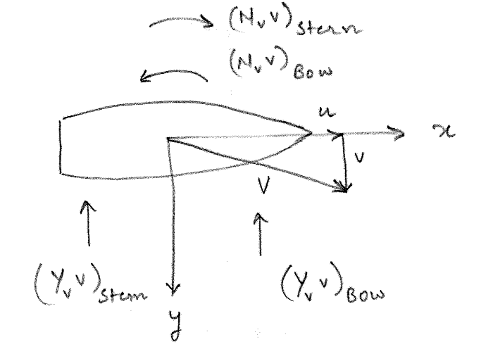
Both bow and stern components of the hydrodynamic force will act in the same direction that is opposite to the sway velocity \(v\). These forces are caused by the fluid moving past the hull in the transverse direction. Note that the total sway force is given by
\[\begin{align} Y = (Y_vv)_{bow} + (Y_vv)_{stern} + \text{Other nonlinear components} \end{align}\]
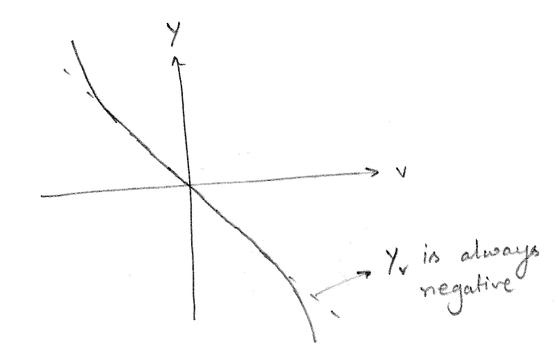
The plot of \(Y\) vs \(v\) is seen in Figure 4.5. It can be seen that close to \(v=0\), the slope of the graph will be negative as a positive sway velocity will result in a negative sway force. The slope of this curve at the origin is the hydrodynamic derivative \(Y_v\). As both bow and stern components reinforce in the same direction, the hydrodynamic derivative \(Y_v\) will always be negative and have a large magnitude.
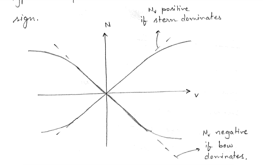
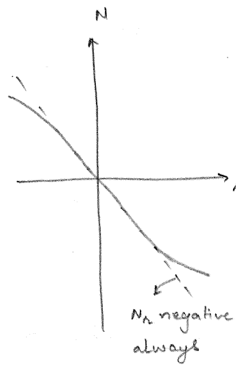
A sway velocity as shown in Figure 4.4 will also result in a yaw moment due to asymmetry of the forward and aft regions of the vessel. It is easy to see that the hydrodynamic force due to the stern \((Y_vv)_{stern}\) will result in a positive yaw moment \((N_vv)_{stern}\) about the amidships of the vessel. On the other hand the hydrodynamic force due to the bow \((Y_vv)_{bow}\) will result in a negative yaw moment \((N_vv)_{bow}\) about the amidships of the vessel. The net yaw moment on the vessel will be the difference between the contributions from bow and stern. Thus, \(N_v\) for a typical ship will be small in magnitude and of uncertain sign. A plot of \(N\) vs \(v\) is seen in Figure 4.6.
A similar argument holds for the sway acceleration derivatives too. Thus, \(Y_{\dot{v}}\) will always be negative and have a large magnitude while \(N_{\dot{v}}\) for a typical ship will be small in magnitude and of uncertain sign.
4.7.2 Pure Yaw Hydrodynamic Derivatives
Let us now consider the case where the vessel experiences pure yaw about the BCS origin with \(v = \dot{v} = 0\), \(\dot{r}=0\) and \(r \neq 0\) as seen in Figure 4.7. In this case, the forward region of the vessel will be experiencing starboard velocity that increases from the BCS origin towards the bow. Similarly, the stern region of the vessel will be experiencing port velocity that increases in magnitude from the BCS origin towards the stern.
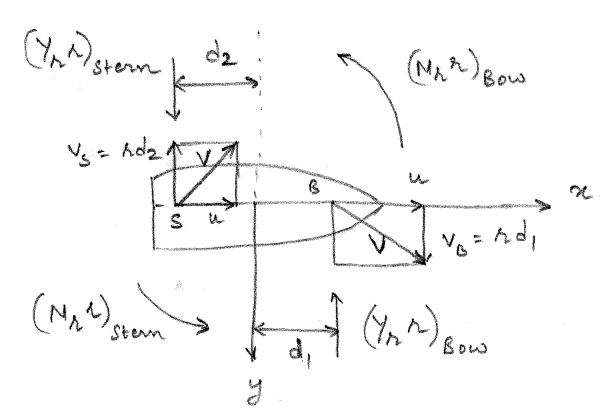
The resultant linearized force acting on the forward portion of the hull \((Y_rr)_{bow}\) is assumed to act notionally at point \(B\). The resultant linearized force acting on the stern potion of the hull \((Y_rr)_{stern}\) is assumed to act notionally at point \(S\). It can be seen that the sway hydrodynamic force due to bow and stern will oppose each other. However, the yaw hydrodynamic moment due to the bow and stern components will complement each other.
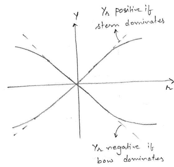
Thus, \(Y_r\) for a typical ship small in magnitude and of uncertain sign. However, \(N_r\) for a typical ship will always be negative and large. The typical plot of \(Y\) vs \(r\) and \(N\) vs \(r\) are shown in Figure 4.8 and Figure 4.9 respectively.
A similar argument holds for the yaw acceleration derivatives too. Thus, \(N_{\dot{r}}\) will always be negative and have a large magnitude while \(Y_{\dot{r}}\) for a typical ship will be small in magnitude and of uncertain sign.
4.7.3 Mass and Inertia Terms
Some of the other quantities appearing in the constants \(A\), \(B\) and \(C\) are \(x_G\), \(m\) and \(I_z\). The mass \(m\) and yaw mass moment of inertia \(I_z\) are large and positive. The location of center of gravity \(x_G\) with respect to amidships is usually small and of uncertain sign.
4.8 Qualitative Assessment of Stability
Based on the qualitative assessment described in the last section and the magnitudes and signs of the constants \(A\), \(B\) and \(C\) can be ascertained. From \(\eqref{eq-A}\) it can be seen that the first term \((m - Y_{\dot{v}})(I_z - N_{\dot{r}})\) is product of two large positive numbers and dominates the other term \((Y_{\dot{r}} - m x_G)(N_{\dot{v}} - m x_G)\), which is a product of smaller numbers of uncertain sign. Thus it can be concluded that for a typical ship \(A>0\). Similarly from \(\eqref{eq-B}\), the sign of \(B\) is dominated by the first two terms \(-(I_z - N_{\dot{r}})Y_v\) and \(-(m - Y_{\dot{v}})(N_r - mx_GU)\). Thus for a typical ship \(B>0\).
Thus the stability conditions shown in \(\eqref{eq-neg-real-root-condition-1}\) and \(\eqref{eq-neg-real-root-condition-2}\) reduces to \(\eqref{eq-stability-criterion}\). \(C\) is therefore also known as the stability constant.
\[\begin{align} C = (N_r - mx_GU) Y_v - (Y_r - mU) N_v > 0 \label{eq-stability-criterion} \end{align}\]
More positive \(C\) means that the ship will be very stable and will require considerable effort to turn. More negative \(C\) means that the ship will be more unstable and require continuous use of rudder to keep course. Also one can observe that \(x_G>0\) (center of gravity forward of amidships) leads to more stability.
The inequality shown in \(\eqref{eq-stability-criterion}\) can also be expressed as shown in \(\eqref{eq-stability-lever-arm}\)
\[\begin{align} \frac{N_r - mx_GU}{Y_r - mU} > \frac{N_v}{Y_v} \label{eq-stability-lever-arm} \end{align}\]
where the stability is shown in terms of comparison of the lever arms of the hydrodynamic forces on the hull in the case of pure yaw and pure sway. Based on the qualitative analysis of the previous section, it can be deduced that for typical ships \(N_r - mx_GU < 0\), \(Y_r - mU < 0\) and \(Y_v < 0\). If \(N_v\) is positive, stability is assured. If \(N_v\) is negative, as is for fine form ships with fuller stern and a lean long bow, the ship will not be straight line stable.
4.9 Exercises
A ship is disturbed from its straight line path by a momentary gust of wind. After the disturbance, the ship settles into a new straight line path at a \(10^\circ\) angle to its original course. What type of stability does this ship demonstrate? Explain your reasoning.
Consider a modern container ship with the following characteristics:
- \(Y_v\) is large and negative
- \(N_r\) is large and negative
- \(N_v\) is small and negative
- \(Y_r\) is small and negative
- \(x_G\) is small and positive
- Is this vessel likely to be straight-line stable? Why or why not? Explain your reasoning.
- If the center of gravity of the vessel is moved aft, how will this affect the stability?
A ship has the following non-dimensional hydrodynamic derivatives and characteristics:
- \(Y_v' = -0.35\)
- \(Y_r' = -0.12\)
- \(N_v' = -0.05\)
- \(N_r' = -0.15\)
- \(m' = 0.72\)
- \(x_G' = 0.1\)
Calculate the non-dimensional stability constant \(C'\) and determine if the ship is straight-line stable.
If the center of gravity of the ship is moved aft so that \(x_G = -0.1\), is the ship still straight-line stable?
If the ship described in the previous question is \(180\) m long, determine the location of the center of gravity from the midship where the ship will just lose its straight-line stability.
Consider two identical ships, except that Ship A has its cargo loaded primarily in the forward section while Ship B has its cargo loaded primarily in the aft section. During sea trials, the following observations were made:
- Ship A maintains course more easily and requires fewer rudder corrections than Ship B
- When both ships are subjected to the same wind gust, Ship B takes longer to settle into a new straight path
Using the concepts of straight-line stability and the stability criterion, explain:
- Why does Ship A require fewer rudder corrections?
- Why does Ship B take longer to settle after a disturbance?
- If you were advising on cargo loading for better course-keeping, what would you recommend and why?
What is the likely stability behavior of the following ships? Explain your reasoning.
- A modern container ship that is characterized by a fine form bow and a fuller transom stern.
- A modern oil tanker that is characterized by a full form bow as compared to the stern.
Why do the container ship and the oil tanker have different designs as described above?
A ship model has the following non-dimensional hydrodynamic derivatives:
- \(Y_v' = -0.42\)
- \(Y_r' = -0.15\)
- \(N_v' = -0.08\)
- \(N_r' = -0.18\)
- \(m' = 0.85\)
- \(x_G' = 0.05\)
- Calculate the non-dimensional stability constant \(C'\).
- If the ship is found to be unstable, what is the minimum change needed in \(N_v'\) to make it stable while keeping all other parameters constant?
Two identical ships have different cargo loading conditions resulting in different longitudinal centers of gravity. Ship A has \(x_G' = 0.08\) and Ship B has \(x_G' = -0.06\). Other parameters are:
- \(Y_v' = -0.38\)
- \(Y_r' = -0.14\)
- \(N_v' = -0.06\)
- \(N_r' = -0.16\)
- \(m' = 0.78\)
Calculate and compare the stability constants for both ships. Which ship is more stable?
A ship designer wants to ensure straight-line stability by modifying the hull form to adjust \(N_v'\). The ship has:
- \(Y_v' = -0.45\)
- \(Y_r' = -0.16\)
- \(N_r' = -0.20\)
- \(m' = 0.90\)
- \(x_G' = 0.04\)
What is the maximum negative value that \(N_v'\) can have while still maintaining straight-line stability?
A ship has a length of \(200\) m and the following non-dimensional parameters:
- \(Y_v' = -0.40\)
- \(Y_r' = -0.13\)
- \(N_v' = -0.07\)
- \(N_r' = -0.17\)
- \(m' = 0.82\)
- Calculate the range of \(x_G'\) values for which the ship will be straight-line stable.
- Convert this range to actual distances from midship in meters.
A ship has the following non-dimensional parameters at its design speed of \(20\) knots:
- \(Y_v' = -0.32\)
- \(Y_r' = -0.11\)
- \(N_v' = -0.04\)
- \(N_r' = -0.14\)
- \(m' = 0.75\)
- \(x_G' = 0.06\)
The ship is found to be marginally stable at this speed. At what speed will the ship become unstable if all other parameters remain constant? Express your answer as the largest integer less than the critical speed in knots.
A vessel operating at \(15\) knots has the following non-dimensional parameters:
- \(Y_v' = -0.35\)
- \(Y_r' = -0.12\)
- \(N_v' = -0.05\)
- \(N_r' = -0.13\)
- \(m' = 0.75\)
- \(x_G' = -0.01\)
Assuming that the dimensional hydrodynamic derivatives do not vary significantly with speed within the speed range considered (this is an unusual assumption, but we will make it for this problem), calculate:
- The stability constant at \(15\) knots
- The critical speed at which the vessel will lose stability
- The stability margin at \(15\) knots (defined as the difference between critical and operating speeds)
A ship designer is working on a vessel that needs to maintain straight-line stability up to a maximum speed of \(25\) knots. The vessel has:
- \(Y_v' = -0.35\)
- \(Y_r' = -0.12\)
- \(N_r' = -0.15\)
- \(m' = 0.78\)
- \(x_G' = 0.04\)
- Current \(N_v' = -0.06\)
What is the minimum value of \(N_v'\) (including a margin of \(0.01\)) needed to ensure straight-line stability up to \(25\) knots?
Answer Key
This ship demonstrates straight line stability. The key characteristics that indicate this are:
- The ship returns to a straight line path after the disturbance
- The new path is at an angle (10°) to the original course
- The ship does not return to its original heading This matches the definition of straight line stability where the final path is straight but not necessarily in the same direction as the initial path.
For the modern container ship:
Straight-line stability analysis:
- The stability criterion is \(C = (N_r - mx_GU) Y_v - (Y_r - mU) N_v > 0\)
- Given: \(Y_v\) is large and negative, \(N_r\) is large and negative, \(N_v\) is small and positive, \(Y_r\) is small and negative, \(x_G\) is small and positive
First term: \((N_r - mx_GU) Y_v\)
- \(N_r\) is large negative and \(Y_v\) is large negative
- Their product will be large positive
- The \(-mx_GU\) term aids in increasing \((N_r - mx_GU)Y_v\)
- Overall, this term remains significantly positive
Second term: \(-(Y_r - mU) N_v\)
- Since \(N_v\) is negative and small
- \((Y_r - mU)\) is negative (as \(mU\) dominates over small \(Y_r\))
- Their product, when negated, gives a small negative contribution
Therefore, C is positive, indicating straight-line stability.
Moving the center of gravity aft (decreasing \(x_G\)):
- In the first term, \(-mx_GU Y_v\) becomes more negative as \(x_G\) decreases (since \(Y_v\) is negative)
- This decreases the value of \((N_r - mx_GU)Y_v\)
- The second term \(-(Y_r - mU)N_v\) is unaffected by \(x_G\)
- The overall effect is a reduction in C, making the vessel less stable
- This shows that moving weight aft tends to reduce straight-line stability
Non-dimensional stability constant \(C' = 0.0357\) \(> 0\) and the ship is straight-line stable
For \(x_G' = -0.10\), non-dimensional stability constant \(C' = -0.0147\) \(< 0\) and the ship is not straight-line stable
The ship will just lose its straight-line stability when \(x_G' = -0.0417\)
The location of the center of gravity from the midship is \(-7.50\) m
Ship A requires fewer rudder corrections because it has a higher stability constant \(C\).
Ship B takes longer to settle after a disturbance because it has a lower stability constant \(C\).
If you were advising on cargo loading for better course-keeping, you would recommend loading the cargo in the aft section of the ship. This would increase the stability constant \(C\) and make the ship more stable.
The container ship is likely to be straight-line stable because it has a fuller stern and a lean long bow, which results in a positive \(N_v\).
The oil tanker is likely to be unstable because it has a full form bow as compared to the stern, which results in a negative \(N_v\).
The container ship and the oil tanker have different designs as described above because the container ship is designed for faster speeds and carries cargo with less density while the oil tanker carries relatively dense crude oil or its derivatives and needs a fuller form to maximize the cargo that can be carried.
Non-dimensional stability constant \(C' = 0.0134\) \(> 0\)
Minimum \(N_v'\) required for stability: \(-0.0934\)
Change needed in \(N_v'\): \(-0.0134\)
Ship A stability constant \(C_A' = 0.0293\)
Ship B stability constant \(C_B' = -0.0122\)
Ship A is more stable.
Maximum negative value of \(N_v'\) for stability: \(-0.1002\)
For straight-line stability: \(x_G' > -0.0046\)
Distance from midship: \(x_G > -0.91\) m
The ship will become unstable at speeds below \(19.0\) knots
Stability constant at 15 knots: \(C' = 0.0064\)
Critical speed: \(17.4\) knots
Stability margin: \(2.4\) knots
Minimum required \(N_v'\) for stability: \(-0.0605\)