11 Performance Metrics for Control System Design
This chapter will focus on the performance metrics for control systems. Particularly, the first order and second order systems will be discussed. The contours of the performance characteristics on the complex \(s\)-plane will be discussed. Finally, the design process of a control engineer to satisfy the specified metrics will be reviewed.
11.1 First Order System
A first order differential system is governed by a first order differential equation. A generic form of this differential equation is shown in
\[\begin{align} \dot{x} + a x = bu \end{align}\]
where \(u\) is the control input and \(x\) is the scalar state being controlled. The transfer function for this system is given by
\[\begin{align} G(s) = \frac{X(s)}{U(s)} = \frac{b}{s+a} \end{align}\]
Assuming that the input is a step function (Heaviside function) \(U(s) = \frac{1}{s}\), the response \(X(s)\) in its partial fraction decomposition is given by
\[\begin{align} X(s) = \frac{b}{s(s+a)} = \frac{b}{a} \left\{\frac{1}{s} - \frac{1}{s+a}\right\} \end{align}\]
Taking a inverse Laplace transform yields,
\[\begin{align} x(t) = \frac{b}{a} \left(1 - e^{-at}\right) \end{align}\]
When \(b=a\),
\[\begin{align} x(t) = \left(1 - e^{-at}\right) \end{align}\]

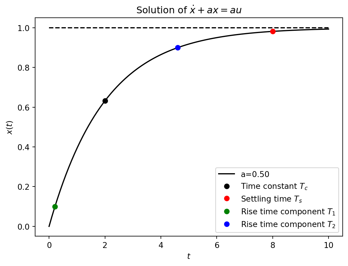
The plot of the response \(x(t)\) is shown in Figure 11.1. The metrics that characterize the response of a first order system are:
- Time constant: The time constant \(T_c\) is defined as the time it takes for the system to reach \(\left(1 - \frac{1}{e}\right) \approx 63\%\) of the steady state value. By applying this definition as seen in \(\eqref{eq-time-constant-def}\) it can be seen that the time constant is given by \(\eqref{eq-time-constant-first}\).
\[\begin{align} x(T_c) = 1 - e^{-aT_c} = 1 - \frac{1}{e} \approx 63\% \label{eq-time-constant-def} \end{align}\]
\[\begin{align} T_c = \frac{1}{a} \label{eq-time-constant-first} \end{align}\]
- Rise time: The rise time \(T_r\) is defined as the time it takes for the system to go from \(10\%\) of the steady state value to \(90\%\) of the steady state value. The rise time is a measure of how fast the system responds to a change in input. Mathematically, it is defined as shown below
\[\begin{align} T_r = T_2 - T_1 \text{ where } x(T_2) = 0.9 \text{ and } x(T_1)=0.1 \end{align}\]
- Settling time: The settling time \(T_s\) is defined as the time it takes the system to stabilize to within \(2\%\) of the steady state value (\(x(T_s) = 0.98\)). Mathematically, it can be shown that
\[\begin{align} T_s \approx 4 T_c = \frac{4}{a} \end{align}\]
11.2 Second Order System
A second order system is governed by a second order differential equation. A generic form of this differential equation is shown below.
\[\begin{align} \ddot{x} + b \dot{x} + c x = au \end{align}\]
The transfer function for this second order system is given by
\[\begin{align} G(s) = \frac{X(s)}{U(s)} = \frac{a}{s^2 + bs + c} \end{align}\]
Since the denominator of the transfer function is a quadratic polynomial in \(s\), the system will have two poles. There are four different possibilities that can occur:
- Real and distinct roots
- Real repeated roots
- Pair of imaginary roots
- Complex roots
The response of the system to a step input \(U(s) = \frac{1}{s}\) in the above four conditions is discussed below.
11.2.1 Real and Distinct Roots
In this case, the poles of the system are real and distinct. Assuming the roots to be \(s=r_1\) and \(s=r_2\), the denominator of the transfer function \(G(s)\) can be expressed as \(D(s) = s^2 + bs + c = (s - r_1)(s - r_2)\). The partial fraction decomposition of the response \(X(s)\) can be expressed as
\[\begin{align} X(s) = \frac{a}{s(s^2+bs+c)} = \frac{A}{s} + \frac{B}{s-r_1} + \frac{C}{s-r_2} \end{align}\]
Thus the response \(x(t)\), obtained by inverse Laplace transform, is given by
\[\begin{align} x(t) = A + B e^{r_1 t} + C e^{r_2 t} \end{align}\]
The constants \(A\), \(B\) and \(C\) are determined by the initial conditions. If \(r_1<0\) and \(r_2<0\) then the system is stable as the exponential terms will decay with time and the system achieves steady state. Such a system is called an overdamped system.
If \(r_1>0\) or \(r_2>0\) then the system response grows unboundedly.
11.2.2 Real and Repeated Roots
In this case, the poles of the system are real and repeated. Assuming the repeated root to be \(s=r\), the denominator of the transfer function \(G(s)\) can be expressed as \(D(s) = s^2 + bs + c = (s - r)^2\). The partial fraction decomposition of the response \(X(s)\) can be expressed as
\[\begin{align} X(s) = \frac{a}{s(s^2+bs+c)} = \frac{A}{s} + \frac{B}{s-r} + \frac{C}{(s-r)^2} \end{align}\]
Thus the response \(x(t)\), obtained by inverse Laplace transform, is given by
\[\begin{align} x(t) = A + B e^{r t} + C te^{r t} \label{eq-repeated-root-time-domain} \end{align}\]
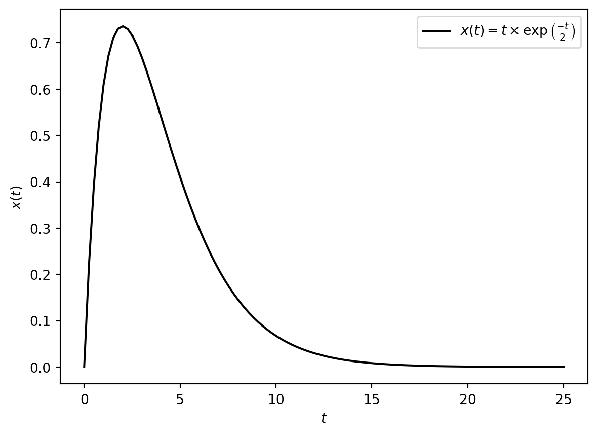
The constants \(A\), \(B\) and \(C\) are determined by the initial conditions. If \(r<0\) then the system is stable as the exponential terms will decay with time and the system reaches a steady state response. Note that the third term \(C te^{r t}\) too will decay with time as exponential term decays at a faster rate than the linear term. Figure 11.2 shows the decay of \(te^{\frac{-t}{2}}\) with time and corresponds to the third term in \(\eqref{eq-repeated-root-time-domain}\) for the case \(r=\frac{-1}{2}\). A second order system with repeated real roots with \(r<0\) is known as critically damped system.
If instead \(r>0\) then the response grows unboundedly.
11.2.3 Pair of Imaginary Roots
In this case, the poles of the system are purely imaginary. For \(b=0\) and \(c>0\), the roots are \(s=i\sqrt{c}=i\omega_n\) and \(s=-i\sqrt{c}=-i\omega_n\). In this case the denominator of the transfer function \(G(s)\) can be expressed as \(D(s) = s^2 + c = (s^2 + \omega_n^2)\). The partial fraction decomposition of the response \(X(s)\) can be expressed as
\[\begin{align} X(s) = \frac{a}{s(s^2+c)} = \frac{A}{s} + \frac{Bs+C}{s^2 + \omega_n^2} \end{align}\]
Thus the response \(x(t)\), obtained by inverse Laplace transform, is given by
\[\begin{align} x(t) = A + B \cos(\omega_n t) + \frac{C}{\omega_n} \sin(\omega_n t) \end{align}\]
The constants \(A\), \(B\) and \(C\) are determined by the initial conditions. It can be seen that in this case, the response \(x(t)\) exhibits an oscillatory transient motion with frequency \(\omega_n\) about a mean value and the oscillations do not decay with time. However, the response does not grow unboundedly either. A second order system with a pair of imaginary roots is known as an undamped system and its response is known as undamped response.
11.2.4 Complex Roots
In this case the poles of the system are complex. Assuming the roots to be \(s=\sigma\pm i\omega_d\) the denominator of the transfer function \(G(s)\) can be expressed as \(D(s) = s^2 + bs + c = (s-\sigma)^2 + \omega_d^2\). The partial fraction decomposition of the response \(X(s)\) can be expressed as
\[\begin{align} X(s) = \frac{a}{s(s^2+bs+c)} = \frac{A}{s} + \frac{Bs + C}{(s-\sigma)^2 + \omega_d^2} \end{align}\]
Thus the response \(x(t)\), obtained by inverse Laplace transform, is given by
\[\begin{align} x(t) = A + B e^{\sigma t} \cos(\omega_d t) + \left(\frac{B\sigma + C}{\omega_d}\right) e^{\sigma t} \sin(\omega_d t) \end{align}\]
The constants \(A\), \(B\) and \(C\) are determined by the initial conditions. In this case the response \(x(t)\) exhibits an oscillatory behavior with frequency \(\omega_d\) modulated by \(e^{\sigma t}\). If \(\sigma < 0\) then the last two terms of the response decay with time and the system will reach steady state. Such a system is called an under-damped system.
Defining \(\omega_n^2 = c\), \(K = \frac{a}{c}\) and \(\zeta = \frac{b}{2\sqrt{c}}\), the Laplace transform of the response \(X(s)\) for a step input \(U(s) = \frac{1}{s}\) becomes
\[\begin{align} X(s) = \frac{K\omega_n^2}{s(s^2 + 2\zeta\omega_ns + \omega_n^2)} \end{align}\]
Separating it into partial fractions and assuming \(\zeta < 1\) yields
\[\begin{align} X(s) &= K\left[\frac{1}{s} - \frac{s + 2\zeta\omega_n}{s^2 + 2\zeta\omega_ns + \omega_n^2}\right] \nonumber \\ &= K\left[\frac{1}{s} - \frac{s + \zeta\omega_n}{(s + \zeta \omega_n)^2 + \omega_n^2(1-\zeta^2)} \right. \nonumber\\ & \qquad \left. -\frac{\zeta\omega_n}{\omega_n\sqrt{1 - \zeta^2}}\frac{\omega_n\sqrt{1 - \zeta^2}}{(s + \zeta \omega_n)^2 + \omega_n^2(1-\zeta^2)}\right] \end{align}\]
Taking an inverse Laplace transform yields \(x(t)\) as
\[\begin{align} x(t) &= K\left[1 - e^{-\zeta \omega_n t} \cos\left(\left(\omega_n\sqrt{1 - \zeta^2}\right)t\right) \right.\nonumber\\ &\qquad \left.- \frac{\zeta}{\sqrt{1 - \zeta^2}} e^{-\zeta \omega_n t} \sin\left(\left(\omega_n\sqrt{1 - \zeta^2}\right)t\right)\right] \nonumber\\ &= K\left[1 - \frac{e^{-\zeta \omega_n t}}{\sqrt{1 - \zeta^2}} \left\{\sqrt{1 - \zeta^2} \cos\left(\left(\omega_n\sqrt{1 - \zeta^2}\right)t\right) \right.\right.\nonumber\\ &\qquad \left.\left.- \zeta \sin\left(\left(\omega_n\sqrt{1 - \zeta^2}\right)t\right)\right\}\right] \nonumber\\ &= K\left[1 - \frac{e^{-\zeta \omega_n t}}{\sqrt{1 - \zeta^2}} \cos\left(\omega_dt - \phi\right)\right] \label{eq-normalized-response} \end{align}\]
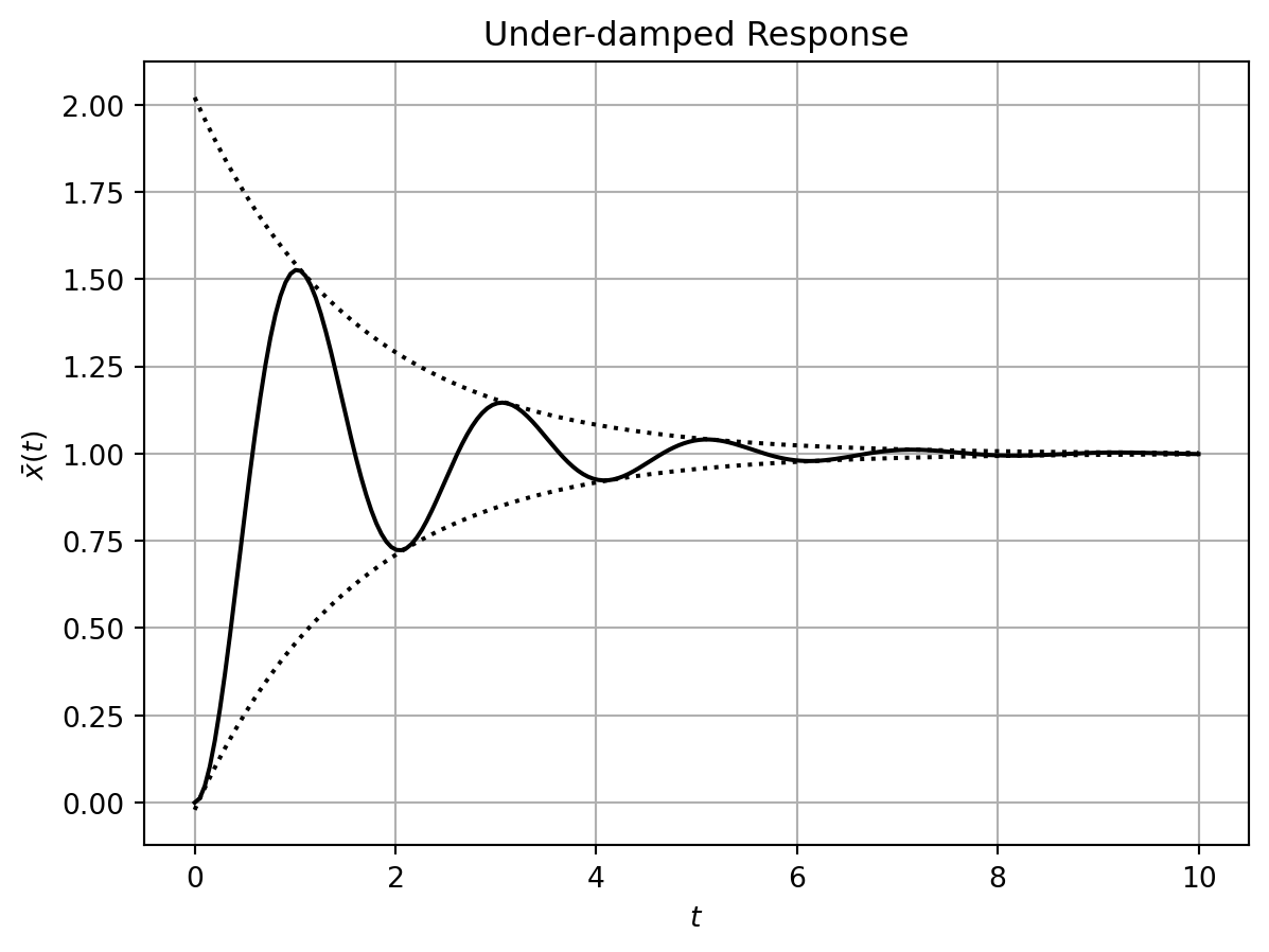
where \(\omega_d = \omega_n \sqrt{1 - \zeta^2}\), \(\cos(\phi) = \sqrt{1 - \zeta^2}\) and \(\sin(\phi) = \zeta\). The normalized response \(\bar{x}(t) = x(t) / K\) is plotted in Figure 11.3.
The metrics that characterize the under-damped response of a second order system are:
- Settling time
- Peak time
- Maximum overshoot
- Rise time
Settling Time: Settling time \(T_s\) is the time it takes for the response amplitude to settle within \(2\%\) of the steady state value. If the envelope response (seen as the dotted lines in Figure 11.3) is denoted by \(x_e(t)\) then the settling time is mathematically defined as
\[\begin{align} x_e(T_s) = 0.98 \\ 1 - \frac{e^{-\zeta \omega_n T_s}}{\sqrt{1 - \zeta^2}} = 0.98 \end{align}\]
Rearranging the above equation yields the settling time as shown in \(\eqref{eq-settling-time-2}\)
\[\begin{align} T_s = - \frac{\ln\left(0.02 \sqrt{1 - \zeta^2}\right)}{\zeta \omega_n} \label{eq-settling-time-2} \end{align}\]
For \(0 \leq \zeta \leq 0.9\), the numerator in \(\eqref{eq-settling-time-2}\) does not vary significantly (\(3.9 \leq -\ln\left(0.02 \sqrt{1 - \zeta^2}\right) \leq 4.7\)). Thus, the settling time can be approximated as
\[\begin{align} T_s \approx \frac{4}{\zeta \omega_n} = 4\tau \label{eq-settling-time-approx} \end{align}\]
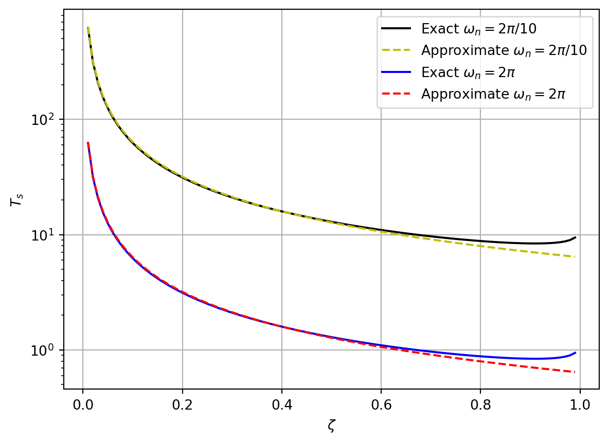
where \(\tau = \frac{1}{\zeta \omega_n}\) is the time constant of the system. A comparison of the exact and approximate expressions for the settling time for two different values of \(\omega_n\) is shown in Figure 11.4.
Peak Time: Peak time \(T_p\) is defined as the time at which the peak of the response occurs. Taking a derivative of \(\eqref{eq-normalized-response}\) yields the normalized velocity as shown below.
\[\begin{align} \dot{\bar{x}}(t) &= e^{-\zeta \omega_n t} \frac{\zeta \omega_n}{\sqrt{1 - \zeta^2}} \cos\left(\omega_dt - \phi\right) + \frac{e^{-\zeta \omega_n t}}{\sqrt{1 - \zeta^2}} \omega_d \sin\left(\omega_dt - \phi\right) \nonumber \\ &= e^{-\zeta \omega_n t} \frac{\omega_n}{\sqrt{1 - \zeta^2}} \left\{\sin(\phi) \cos\left(\omega_dt - \phi\right) + \cos(\phi)\sin\left(\omega_dt - \phi\right)\right\} \nonumber\\ &= e^{-\zeta \omega_n t} \frac{\omega_n}{\sqrt{1 - \zeta^2}} \sin(\omega_dt) \label{eq-normalized-velocity} \end{align}\]
At the peak time \(t=T_p\), the velocity \(\dot{\bar{x}}(T_p) = 0\). Thus the time of the first peak after \(t=0\) happens at
\[\begin{align} T_p = \frac{\pi}{\omega_d} = \frac{\pi}{\omega_n \sqrt{1 - \zeta^2}} \label{eq-peak-time-2} \end{align}\]
Maximum Overshoot: The maximum overshoot \(M_p\) is defined as a percentage of the steady state value. Thus it is obtained from the value of the normalized response \(\bar{x}(t)\) at \(t=T_p\). The maximum overshoot is mathematically given by
\[\begin{align} \bar{x}(T_p) &= 1 + M_p \nonumber\\ &= 1 - \frac{e^{-\zeta \omega_n T_p}}{\sqrt{1 - \zeta^2}} \cos\left(\pi - \phi\right) \nonumber\\ &= 1 + e^{-\frac{\pi \zeta}{\sqrt{1 - \zeta^2}}} \end{align}\]
Thus, the maximum overshoot is given by
\[\begin{align} M_p = e^{-\frac{\pi \zeta}{\sqrt{1 - \zeta^2}}} \label{eq-max-overshoot} \end{align}\]
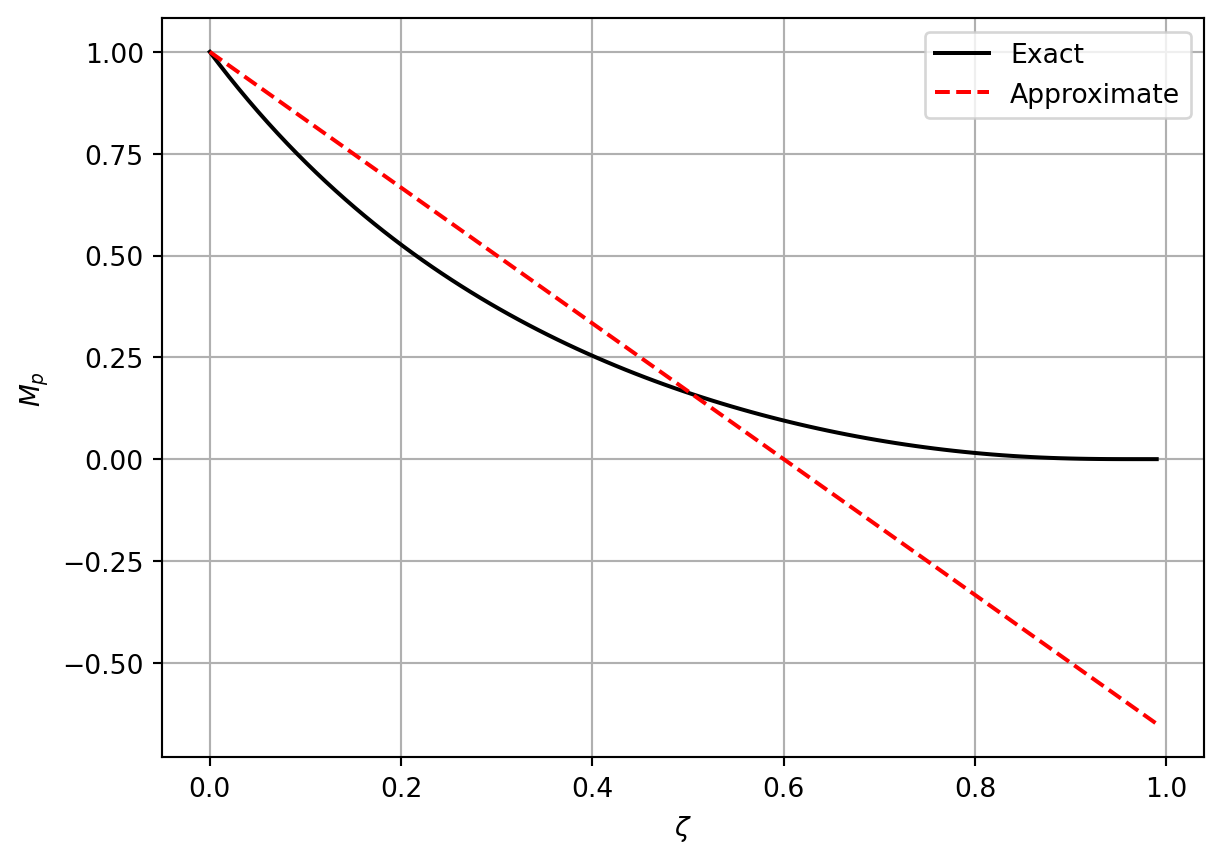
For \(0 \leq \zeta \leq 0.5\), the overshoot can be approximated as
\[\begin{align} M_p = 1 - \frac{\zeta}{0.6} \label{eq-max-overshoot-approx} \end{align}\]
A comparison of the original and approximate expression for the overshoot is shown in Figure 11.5
Rise Time: The rise time \(T_r\) is defined as the time it takes for the response to reach the steady state value for the first time. The rise time is mathematically given by
\[\begin{align} \bar{x}(T_r) = 1 \end{align}\]
Substituting \(\eqref{eq-normalized-response}\) into the above equation yields
\[\begin{align} 1 = 1 - \frac{e^{-\zeta \omega_n T_r}}{\sqrt{1 - \zeta^2}} \cos\left(\omega_d T_r - \phi\right) \end{align}\]
It can be seen that the above equation is satisfied when \(\omega_d T_r = \frac{\pi}{2} + \phi\).
\[\begin{align} \tan\left(\omega_d T_r\right) = \frac{-1}{\tan(\phi)} = -\frac{\sqrt{1 - \zeta^2}}{\zeta} \end{align}\]
Solving the above equation for \(T_r\) yields
\[\begin{align} T_r = \frac{1}{\omega_d} \left(\frac{\pi}{2} + \phi\right) = \frac{1}{\omega_n \sqrt{1 - \zeta^2}} \left(\frac{\pi}{2} + \sin^{-1}(\zeta)\right) \label{eq-rise-time-2} \end{align}\]
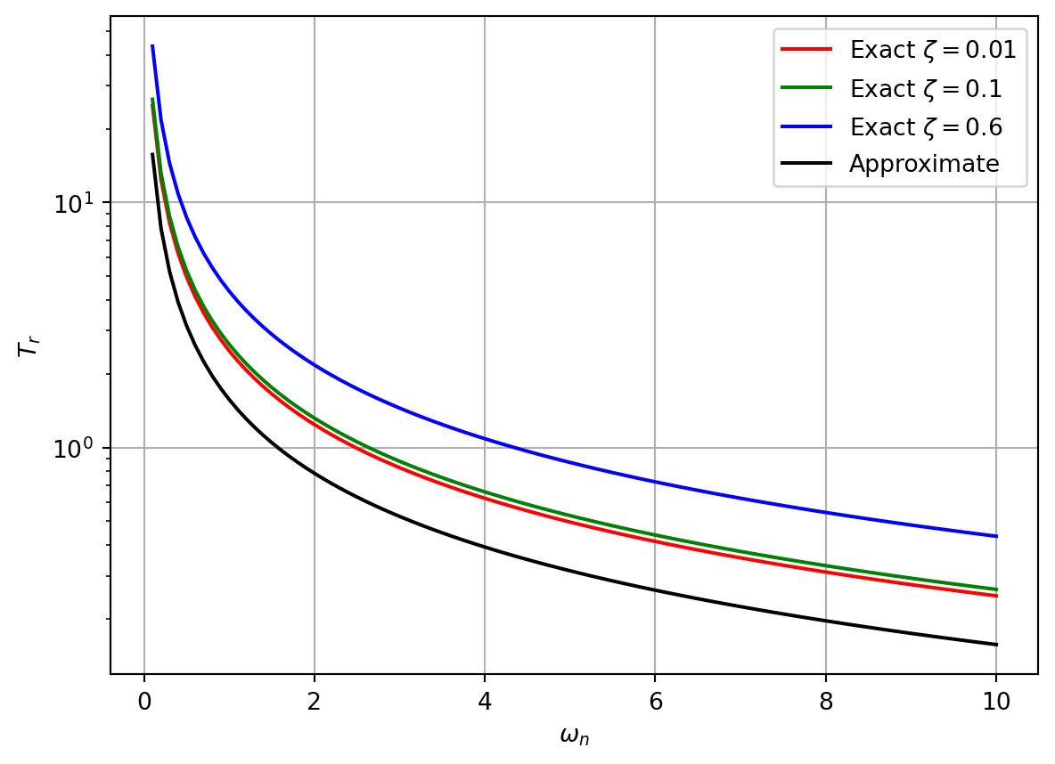
For small values of \(\zeta\), \(\sin^{-1}(\zeta) \approx \zeta\) and \(\omega_d \approx \omega_n\). Thus the rise time can be approximated as
\[\begin{align} T_r \approx \frac{\pi}{2\omega_n} \label{eq-rise-time-approx} \end{align}\]
A comparison of the exact and approximate expressions for the rise time is shown in Figure 11.6.
Summarizing the performance metrics of a second order system, the following table (Table 11.1) can be used to determine the performance metrics for a given \(\zeta\) and \(\omega_n\).
| Metric | Expression | Approximation |
|---|---|---|
| Settling Time | \(T_s = - \frac{\ln\left(0.02 \sqrt{1 - \zeta^2}\right)}{\zeta \omega_n}\) | \(T_s \approx 4\tau = \frac{4}{\zeta \omega_n}\) |
| Peak Time | \(T_p = \frac{\pi}{\omega_d}\) | \(T_p \approx \frac{\pi}{\omega_n}\) |
| Maximum Overshoot | \(M_p = e^{-\frac{\pi \zeta}{\sqrt{1 - \zeta^2}}}\) | \(M_p \approx 1 - \frac{\zeta}{0.6}\) |
| Rise Time | \(T_r = \frac{1}{\omega_d} \left(\frac{\pi}{2} + \phi\right)\) | \(T_r \approx \frac{\pi}{2\omega_n}\) |
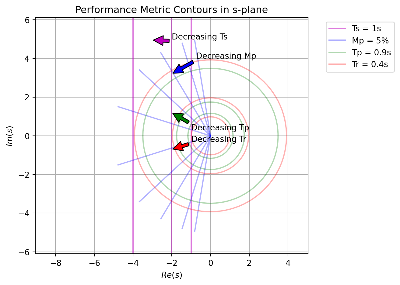
The contour of each performance metric can be plotted in the complex \(s\) plane as shown in Figure 11.7. When designing a control system, the designer can use this plot to determine the region of the complex plane that satisfies all the performance criteria.
